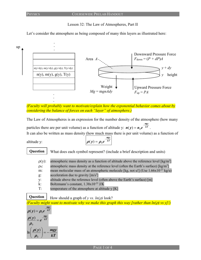
PHYSICS
COURSEWIDE PRELAB HANDOUT
Lesson 32: The Law of Atmospheres, Part II
Let’s consider the atmosphere as being composed of many thin layers as illustrated here:
.
.
.
up
Downward Pressure Force
Fdown = (P + dP)A
Area A
y + dy
n(y+dy), m(y+dy), g(y+dy), T(y+dy)
n(y), m(y), g(y), T(y)
.
.
.
y height
Weight
Mg = mgnAdy
Upward Pressure Force
Fup = PA
(Faculty will probably want to motivate/explain how the exponential behavior comes about by
considering the balance of forces on each “layer” of atmosphere.)
The Law of Atmospheres is an expression for the number density of the atmosphere (how many

mgy
kT
particles there are per unit volume) as a function of altitude y: n( y )  n0 e
.
It can also be written as mass density (how much mass there is per unit volume) as a function of
 ( y)   0 e
altitude y:
Question

mgy
kT
What does each symbol represent? (include a brief description and units)
(y):
0:
m:
g:
y:
k:
T:
atmospheric mass density as a function of altitude above the reference level [kg/m3]
atmospheric mass density at the reference level (often the Earth’s surface) [kg/m3]
mean molecular mass of an atmospheric molecule [kg, not u!] (Use 1.66x10-27 kg/u)
acceleration due to gravity [m/s2]
altitude above the reference level (often above the Earth’s surface) [m]
Boltzmann’s constant, 1.38x10-23 J/K
temperature of the atmosphere at altitude y [K]
How should a graph of y vs. ln() look?
(Faculty might want to motivate why we make this graph this way [rather than ln() vs y]!)
Question
 ( y)   0e

mgy
kT

 ( y)
 e kT
0
mgy
  ( y) 
mgy
  
ln 
kT
 0 
PAGE 1 OF 4
PHYSICS
COURSEWIDE PRELAB HANDOUT
kT   
ln  
mg   0 
kT
kT
y
ln  
ln  0
mg
mg
y  (slope ) x  (intercept )
y
y
ln()
(Faculty can then create/show the Excel graph with just the straight Law of Atm line on it)
What percentage of the sea level atmospheric pressure is the atmospheric
pressure at USAFA (y = 7258 ft = 2212 m)? (Assume an atmosphere at
temperature T = 25 oC.)
Example
P ( y)  P0 e
Question

mgy
kT
 P0 e

( 28.9 u )(1.66 x1027 kg / u )( 9.8 m / s 2 )( 2212m )
(1.38 x10 23 J / K )( 298K )
 0.7766 P0
What does the slope of the y vs. ln() graph depend on?
g, T, and m
y
How would graphs for two different g’s look?
(Sketch and label which is which)
Smaller g
Larger g
ln()
y
How would graphs for two different T’s look?
(Sketch and label which is which)
Larger T
Smaller T
ln()
How would graphs for two gases of different
molecular masses look? (Sketch)
y
Smaller m
Larger m
ln()
What three important assumptions/approximations does the Law of Atmospheres
as stated above use?
Constant g (we assume it doesn’t vary with altitude – but we know it does!)
Constant T (we assume it doesn’t vary with altitude – but measurements show it does!)
Constant m (turbulent mixing says this is constant in the lowest 100 km, but that it
varies above that!)
Question



PAGE 2 OF 4
PHYSICS
COURSEWIDE PRELAB HANDOUT
Let’s deal with each of these assumptions/approximations, one at a time.
Varying “g”
GMm
for the force of gravity on the gas molecules of mass m, rather than
r2
just Fgrav = mg, we can allow for a “g” that varies with altitude. Going through a process similar
to that in the atmosphere handout gives us this expression for density (R = radius of the Earth
and y = altitude above the surface of the Earth, as before):
If we use F grav 
 ( y)   0 e
Question

GMm  1
1 
 

kT  R R  y 
which can also be written as  ( y)   0 e
Why isn’t it correct to just substitute g 

GMm
y
kT R ( R  y )
GM
into the original Law of
r2
Atmospheres expression?
The derivation of the law of atmospheres involves integration with respect to the altitude y. The
expression for “g” includes a hidden “y” in the “r” since r = R+y. We have to integrate correctly
– g isn’t just a constant we can substitute into the final expression.
Question
How would you predict the “correct g” graph of y vs. ln() should look? (Why?)
It should look a bit steeper, because the “corrected g” is actually a little bit smaller than the
uncorrected g.
(Faculty can then show the Excel graph with just the original and the “corrected g” Law of
Atmosphere lines on it)
Question
Why does the “corrected g” graph of y vs. ln() have a slightly more negative
slope (what does that mean, physically)?
The actual “g” decreases as you go up in altitude, so the atmosphere can extend a bit higher
because it isn’t being ‘tugged on’ as much.
Varying “T”
Experimental data (measurements) tell us that T is not constant as you go up in the atmosphere.
Your atmosphere handout shows a temperature profile for just the first 100 km of the
atmosphere, and we have data that extend even higher into the atmosphere.
(Faculty can show the graph that’s in the atmosphere handout [for the first 100 km], then show
the spreadsheet table [and/or graph] of altitude versus T from the MSIS temperature profile in
the spreadsheet [for the first 1000 km].)
Question
When we wanted to incorporate the fact that “g” changes with altitude, what did
we do?
We used an analytic function for “g” and actually found an analytic expression for the
atmospheric density as a function of altitude y.
PAGE 3 OF 4
PHYSICS
Question
COURSEWIDE PRELAB HANDOUT
Why can’t we deal with the varying temperature T in the same way?
We don’t have an analytic function for T as a function of altitude. We just have numerical data
that correspond to different altitudes. We have to treat the altitude in layers, each of which has
its own temperature.
We can allow T to vary, as specified by the data. At every layer (altitude), we can use the
temperature at that altitude to calculate the atmospheric density in a slightly higher layer
(altitude).
Question
Look at the graph of altitude versus temperature. Note that, at higher altitudes,
the temperature rises considerably. What effect do you think this should have on
the y vs. ln() graph? Predict how the graph will change from the one that
assumes a constant (low) T for all the layers of the atmosphere.
The atmospheric density at upper altitudes should be higher than it would be if the temperature
were lower – the atmosphere is more expanded than the constant-low-T model suggests, so
there’s more “stuff” at higher altitudes than the constant-low-T model suggests.
(Faculty can then show the Excel graph with the original, the “corrected g”, and the
“corrected g & T” Law of Atmospheres curves on it.)
Varying “m”
Finally, we also know that the mean mass of the molecules at each altitude doesn’t stay
constant. This is the “m” in the atmospheric density equation. If we allow for the fact that
“turbulent mixing” keeps the mean mass constant for the lowest 100 km of the atmosphere, but
then only the lighter molecules come into play at higher altitudes, we can get a further
correction to the atmospheric density graph. Once again, empirical data (and models) for m as a
function of altitude can be used to treat the layers of the atmosphere.
Question
If lighter molecules can go farther up into the atmosphere than heavier
molecules, how would you expect m to vary with altitude? As you go higher in
the atmosphere, what should happen to m?
The mean mass should become smaller as you go higher.
Question
What effect do you think this should have on the y vs. ln() graph? Predict how
the graph will change from the one that assumes a constant mean mass for all the
layers of the atmosphere.
The atmospheric density at upper altitudes should be even higher than if the mass stayed it its
constant (lower) value. Lighter “stuff” can go higher, so there should be more “stuff” higher.
(Faculty can then show the Excel graph with the original, the “corrected g”, the “corrected g
& T”, and the full MSIS curve (corrected for g, T, and m) Law of Atmospheres curves on it.)
PAGE 4 OF 4