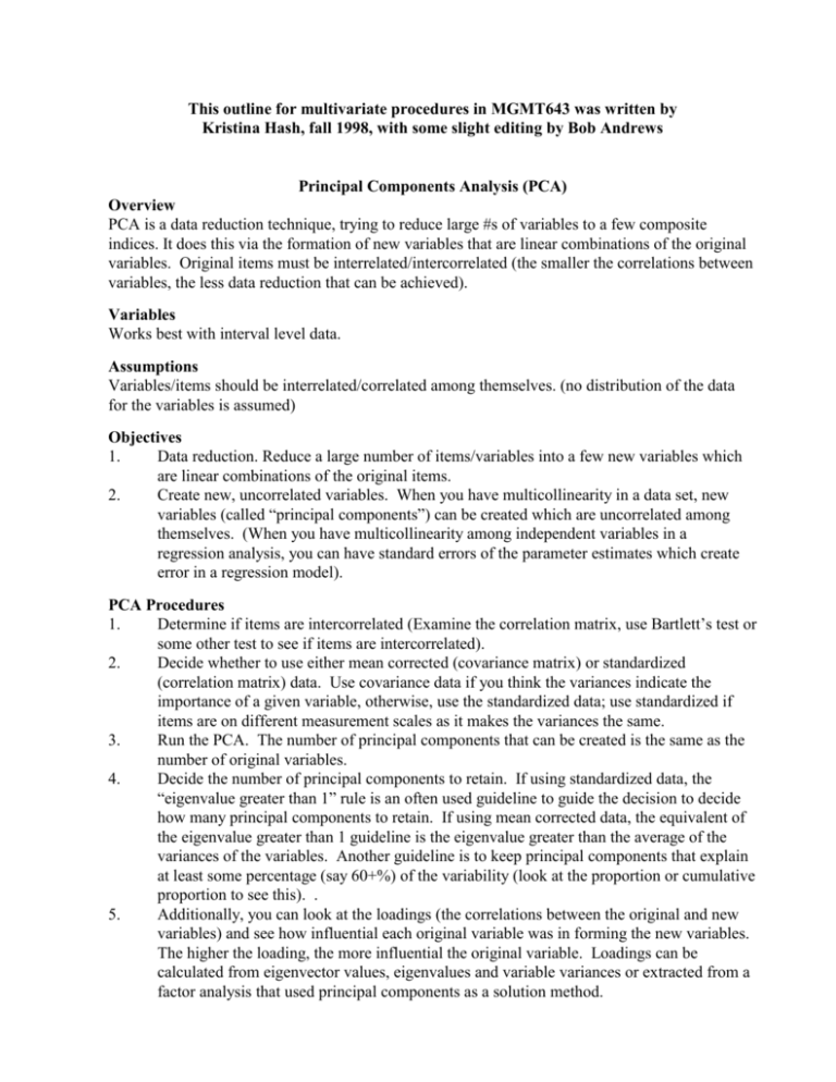
This outline for multivariate procedures in MGMT643 was written by
Kristina Hash, fall 1998, with some slight editing by Bob Andrews
Principal Components Analysis (PCA)
Overview
PCA is a data reduction technique, trying to reduce large #s of variables to a few composite
indices. It does this via the formation of new variables that are linear combinations of the original
variables. Original items must be interrelated/intercorrelated (the smaller the correlations between
variables, the less data reduction that can be achieved).
Variables
Works best with interval level data.
Assumptions
Variables/items should be interrelated/correlated among themselves. (no distribution of the data
for the variables is assumed)
Objectives
1.
Data reduction. Reduce a large number of items/variables into a few new variables which
are linear combinations of the original items.
2.
Create new, uncorrelated variables. When you have multicollinearity in a data set, new
variables (called “principal components”) can be created which are uncorrelated among
themselves. (When you have multicollinearity among independent variables in a
regression analysis, you can have standard errors of the parameter estimates which create
error in a regression model).
PCA Procedures
1.
Determine if items are intercorrelated (Examine the correlation matrix, use Bartlett’s test or
some other test to see if items are intercorrelated).
2.
Decide whether to use either mean corrected (covariance matrix) or standardized
(correlation matrix) data. Use covariance data if you think the variances indicate the
importance of a given variable, otherwise, use the standardized data; use standardized if
items are on different measurement scales as it makes the variances the same.
3.
Run the PCA. The number of principal components that can be created is the same as the
number of original variables.
4.
Decide the number of principal components to retain. If using standardized data, the
“eigenvalue greater than 1” rule is an often used guideline to guide the decision to decide
how many principal components to retain. If using mean corrected data, the equivalent of
the eigenvalue greater than 1 guideline is the eigenvalue greater than the average of the
variances of the variables. Another guideline is to keep principal components that explain
at least some percentage (say 60+%) of the variability (look at the proportion or cumulative
proportion to see this). .
5.
Additionally, you can look at the loadings (the correlations between the original and new
variables) and see how influential each original variable was in forming the new variables.
The higher the loading, the more influential the original variable. Loadings can be
calculated from eigenvector values, eigenvalues and variable variances or extracted from a
factor analysis that used principal components as a solution method.
Factor Analysis (FA)
Overview
Both PCA and FA procedures are data reduction techniques, trying to reduce large #s of variables
to a few composite indices. Both involve the formation of new variables that are linear
combinations of the original variables. Factor analysis goes one step further and tries to determine
an underlying structure or construct. It seeks to explain how certain variables are correlated. Can
be used to develop scales and measure constructs.
Variables
Works best with interval level data.
Assumptions
Multivariate normality only if the maximum likelihood solution method is used; Variables/items
should be interrelated/correlated among themselves
Objectives
1. Identify the smallest # number of factors which best explain or account for the correlations or
covariances among the indicators.
2. Identify, via factor rotations, the most plausible factor solution.
3. Estimate the pattern and structure loadings, communalities, and the unique variances of the
indicators.
4. Provide an interpretation for the common factors.
5. If necessary, estimate the factor scores.
FA Procedures
1.
Use KMO and Bartlett’s test (tests to see if DVs are correlated and data is multivariate
normal) to see if data appropriate for FA (should be significant).
2.
Generation of correlation or covariance matrix.
3.
Extraction of initial factor solution (use PCA) and determine number of factors to keep.
Can use the same guidelines as for PCA such as “eigenvalue greater than one” rule or look
at the cumulative % of variance.
4.
Rotation. Rotation helps achieve a simpler and more interpretable factor structure. Can
use varimax or quartermax or other rotation (use varimax if you do not suspect the
existence of one general factor and use quartermax if you do suspect the presence of one
general factor).
5.
Interpretation. To interpret the factors, you attach labels or meanings to the factors (name
them). To do this, you look at the loadings and identify a pattern among items that load
highly (.6 or .5 and above are often used guidelines) on a particular factor. Factors with
high loadings will have excellent face validity and appear to be measuring some underlying
construct.
6.
Can also go on to construction of scales or factor scores to use in further analysis.
Multivariate Analysis of Variance (MANOVA)
Overview
MANOVA is used to assess the statistical significance of the effect of one or more IVs on a set of
two or more DVs. It is different from ANOVA because ANOVA uses only 1 DV. Use a
MANOVA instead on conducting multiple ANOVAs to control for Type I errors. With
MANOVA, you can see if the vectors of means (centroids) for the groups are significantly
different.
Variables
Involves one or more nominal IVs and 2 or more interval DVs.
Assumptions
Independent observations, multivariate normality (but can violate this especially with an equal
number of observations from each cell or group), equal covariances within IV determined groups
of DVs.
Procedures
1.
Determine whether data meet the assumptions. Can run histograms to check for
multivariate normality and can use Box's M test to determine whether covariances are
equal.
2.
Calculate the test statistic which can be the Hotelling’s T2 (the multivariate version of the
t-test for 2 groups), Pillai's Trace, Wilks Lambda, Hotelling's Trace, or Roy's Largest Root
and look at the significance level. This will show the significance of the effects.
3.
If there is a significant difference among any of the groups then one can further investigate
the nature of this difference by looking at ANOVA results for individual variables,
including Post Hoc Multiple Comparisons for observed means. (In situations with
interrelated variables, individual variables may not be significant.)
4.
If there is a significant difference among any of the groups then one may be able to build a
discriminant function or functions that will allow one to predict group membership for
individual data points. If there is no difference in mean vectors (centroids) for the groups
then it is virtually impossible to build an effective discriminant model.
Discriminant Analysis (DA)
Overview
Discriminant function analysis is used to determine which variables discriminate between two or
more naturally occurring groups and to use those variables to predict group membership of future
cases. It tries to determine whether groups differ with regard to the mean of a variable (similar to
ANOVA/MANOVA). In general, Discriminant Analysis is a very useful tool (1) for detecting the
variables that allow the researcher to discriminate between different (naturally occurring) groups,
and (2) for classifying cases into different groups with a better than chance accuracy. The main
uses of discriminant analysis are (1) to identify variables that are related to group membership and
(2) to predict group membership from a set of predictors.
Variables
DV is nominal and IVs are interval (1 or 2 qualitative dummy variables may be used).
DA Assumptions
Observations for Independent Variables have equal variances and covariances for linear
discriminant functions but quadratic functions can be developed in the case of unequal covariance
matrices. A multivariate normal distribution is assumed for probability estimation.
Equal misclassification costs can be used to adjust prior probabilities in a two group problem to
account for unequal misclassification costs. Consider two groups A & B with prior probabilities
of PA & PB. If C(B|A)/C(A|B)=k then let RA and RB represent the revised prior probabilities where
RA = PA*k/(PA*k + PB) and RB = RB/(PA*k + PB).)
DA Objectives
1.
To identify variables that discriminate best between two or more identifiable groups.
2.
Use the identified variables or factors to develop an equation or function for computing a
new variable or index that will represent differences between the two or more groups.
Conceptually this is equivalent to identifying a new axis and provides maximum separation
between two groups.
3.
Use the identified variables or index to develop a rule to classify future observations into
one of the groups.
DA Procedures
1.
Determine whether data meets the assumptions. Can run histograms to check for
multivariate normality and can use Bartlett’s test to determine whether covariances are
equal. (Estimated posterior probabilities of membership in a group and hypothesis tests are
based on multivariate normality assumptions. Effective discriminant functions may be
developed when the data are not multivariate normal.)
2.
Conduct a MANOVA to see if the vectors of means for the groups are significantly
different. If they are different, this shows that the centroids of the data for the groups differ
significantly. This does not say which variables have different means.
3.
Compute discriminant functions to see which variables should be combined in what way to
discriminate among the groups. (A stepwise discriminant procedure does this
automatically.) Assess the statistical significance to see which variables are most
important. Can use p value of F statistic or of Wilks Lambda to assess significance of a
variable. A low Wilks Lambda, a high F ratio, and a significant p value indicate an
important variable..
4.
Build a model for classifying future cases. Uses stepwise procedures (forward and/or
backward) to decide which variables will be included in the model. These procedures use
the p value or the F statistic to determine whether to include or exclude a variable (see if it
adds significantly to explaining group separation or not).
DA Procedures (continued)
5.
You can then look at the classification results to see what percentage were correctly
classified in using the model. Using the same data to create the discriminant model and to
determine classification results creates what is referred to as the resubstitution error rates.
These tend to underestimate the true error rates for a model. More accurate estimates can
be obtained by predicting group membership for data values that were not used to build the
model, such as classifying a Holdout sample. Another way is via building models by
withholding one data point and then predicting the group for the withheld point and then
repeating this for all data points in the set. The summary error rates are more accurate
(almost unbiased) than the resubstitution rates. This method is referred to as
crossvalidation (SAS & SPSS) or U-Method (Sharma 1996, page 273). The Hold Method
uses one part of the data to build a model and another part to assess the classification
ability of the model. This method requires a large sample size.
Logistic Regression (LR)
Overview
Logistic Regression is an alternative procedure to DA when the dependent variable has only two
groups (as it also can predict group membership) and is an extension of multiple regression. One
can use logistic regression when you violate the normality assumption of DA (either because IVs
are a mix of categorical and continuous variables or because continuous variables are not normally
distributed). Logistic regression is used to predict a dichotomous DV using 1 or more IVs. The
DV usually represents the occurrence or non-occurrence of some outcome event. The procedure
will produce a formula which will predict the probability of the occurrence as a function of the
IVs. It also produces an odds ratio associated with each predictor value. You would use this
instead of linear regression when DV is dichotomous and not continuous. It also differs from
linear regression as it attempts to predict the probability that an observation belongs to each of two
groups as opposed to trying to predict a score on a continuous dependent measure.
Multicollinearity poses similar problems for LR as it does for Ordinary Least Squares Regression.
Variables
A nominal/dichotomous DV with categorical IVs expressed as dummy variables and interval IVs.
LR Assumptions
Independent observations, mutually exclusive and exhaustive categories, specificity (the model
must contain all relevant predictors and no irrelevant predictors).
LR Procedures
1.
Run stepwise logistic regression procedure which will determine statistically significant
predictor variables (uses 2 ). Variables are added or removed based on their likelihood
ratios.
2.
Evaluate the fit of the model using 2 goodness of fit. This compares the observed values
for the subjects in the sample with the predicted values that the subjects should have, based
on the model.
4.
One can also look at the classification table to see how many observations were correctly
predicted, based upon the model. It shows the percent correct.
Cluster Analysis (CA)
Overview
Cluster analysis is a multivariate procedure for detecting natural groupings in data. Cluster analysis
classification is based upon the placing of objects into more or less homogeneous groups, in a
manner such that the relationship between groups is revealed. The two key steps within cluster
analysis are the measurement of distances between objects and the grouping of objects based upon
the resultant distances (linkages). It is different from DA because in DA you already know what
the different groups are, but in CA you are trying to create groups of similar items and do not
know the groups in the beginning.
Variables
Data are to be interval scale measurements.
Assumptions
Since no hypothesis tests are performed or probabilities are estimated, cluster analysis has no
distributional assumptions for the data.
Objectives
1.
Group observations into clusters such that each cluster is as homogeneous (similar,
uniform) as possible with respect to the clustering variables and the groups are as different
as possible.
Procedure
1. Select variables to be used as criteria for cluster formation (select a measure of similarity).
2. Select procedure for measuring distance or similarity between each data point (Euclidean
distance is often used for points) and then between clusters (linkage method). Linkage
methods for hierarchiacal clustering include: Single Linkage or Nearest Neighbor, Complete
Linkage or Furthest Neighbor, Median or Average Linkage, Centroid Method, and Ward’s
Method with each having a different method for measuring distances between clusters.
3. Form clusters (either by using hierarchical clustering or nonhierarchical clustering;
nonhierarchical involves knowing the number of clusters beforehand).
4. Interpret results. This is similar to interpretation in FA as you are naming clusters based upon
similar characteristics, but you are also determining how many clusters exist. One can look at
a dendrogram which shows how items are put together in groups. In this chart one can look at
the distance between the joining of clusters to help decide how many clusters should be used.