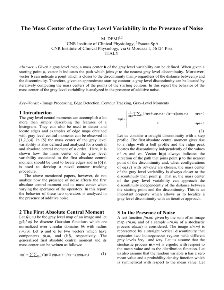
The Mass Center of the Gray Level Variability in the Presence of Noise
M. DEMI1,2
CNR Institute of Clinical Physiology, 2Esaote SpA
CNR Institute of Clinical Physiology, via G.Moruzzi 1, 56124 Pisa
ITALY
1
Abstract: - Given a gray level map, a mass center b of the gray level variability can be defined. When given a
starting point p, vector b indicates the path which joins p to the nearest gray level discontinuity. Moreover,
vector b can indicate a point which is closer to the discontinuity than p regardless of the distance between p and
the discontinuity. Therefore, given an approximate starting contour, a gray level discontinuity can be located by
iteratively computing the mass centers of the points of the starting contour. In this report the behavior of the
mass center of the gray level variability is analyzed in the presence of additive noise.
Key-Words: - Image Processing, Edge Detection, Contour Tracking, Gray-Level Moments
1 Introduction
 1
 e(p) 3 f (p)  g (p,  1 )  f (p  q) qg (q,  3 )

b(p)  

0


e(p)  0
The gray level central moments can accomplish a lot
more than simply describing the features of a
histogram. They can also be used to detect and
locate edges and examples of edge maps obtained
with gray level central moments can be observed in
[1,2,3,4]. In [5] the mass center of the gray level
variability is also defined and analyzed for a central
and absolute central moment of n order. Here, it is
shown how the mass center of the gray level
variability associated to the first absolute central
moment should be used to locate edges and in [6] it
is used to develop a novel contour tracking
procedure.
The above mentioned papers, however, do not
analyze how the presence of noise affects the first
absolute central moment and its mass center when
varying the apertures of the operators. In this report
the behavior of these two operators is analyzed in
the presence of additive noise.
(2)
Let us consider a straight discontinuity with a step
profile. The first absolute central moment gives rise
to a ridge with a bell profile and the ridge peak
locates the discontinuity independently of the values
of 1 and 3. Vector b(p) always indicates the
direction of the path that joins point p to the nearest
point of the discontinuity and, when configurations
of eq.(2) with 1>3/ are chosen, the mass center
of the gray level variability is always closer to the
discontinuity than point p. That is, the mass center
of the gray level variability can approach the
discontinuity independently of the distance between
the starting point and the discontinuity. This is an
important property which allows us to localize a
gray level discontinuity with an iterative approach.
2 The First Absolute Central Moment
3 In the Presence of Noise
Let f(n,m) be the gray level map of an image and let
g(k,l,i) be discrete Gaussian functions which are
normalized over circular domains i with radius
ri=3i. Let p and q be two vectors which have
components (n,m) and (k,l), respectively. The
generalized first absolute central moment and its
mass center can be written as follows:
A test function f(n,m) given by the sum of an image
map s(n,m) and of a sample u(n,m) of a stochastic
process u(n,m) is considered. The image s(n,m) is
represented by a straight vertical discontinuity that
separates two homogeneous regions with different
gray levels levA , and levB. Let us assume that the
stochastic process u(n,m) is ergodic with respect to
the mean value and to the distribution function. Let
us also assume that the random variable u has a zero
mean value and a probability density function which
is symmetrical with respect to the mean value. Let
e(p)  
3
f (p)  g (p, 1 )  f (p  q) g (q, 3 )
(1)
e(p)  0
hu(u) be the probability density function of the
random variable u, then the following notation is
used:
Pa  u  b)   hu (u)du
b
a
E(u   ) a  u  b   (u   )hu (u)du
(3)
b






3 posA
s1 (p)  s(p  q)g (q,  3 )  ( s1 ( )  lev A )GA ( ) Pu  s1  lev A 
3 posB
s1 (p)  s(p  q)g (q,  3 )  ( s1 ( )  lev B )GB ( ) Pu  s1  lev B 
u (p)g (q,  3 )  0
3 posA 1
u (p)g (q,  3 )  0
3 posB 1
3 posA
3 posB
u (p  q)g (q,  3 )  G A ( ) E u u  s1  lev A 
u (p  q)g (q,  3 )  GB ( ) Eu u  s1  lev B 
(6)
a
where
where P{a<u<b} is the probability that a<u(n,m)<b,
 is any scalar value and E{(u-)a<u<b} is the
generalized first moment of the process u(n,m)
computed between the values a and b.
3.1 The Absolute Moment
Due to the presence of the absolute value, the
absolute central moment is obtained by computing
its positive and negative components separately.
e(p)  epos(p)  eneg (p)
(4)
The following relationship is obtained for epos(n,m):
s (p)  s(p  q)g (q, 3 ) 
epos(p)  
3 pos 1
 
u (p)g (q, 3 ) 
3 pos 1
 
u (p  q)g (q, 3 )
3 pos
(5)
where s1(n,m) and u1(n,m) are obtained by
convolving s(n,m) and u(n,m), respectively, with the
Gaussian g(n,m,1). In order to simplify the
calculation of epos(n,m) the domain 3pos is split
into two subdomains 3posA and 3posB: the first
one is the area of 3pos which has gray level levA ,
and the second one is the area of 3pos which has
gray level levB. Let us assume  be the distance of
the point p(n,m) from the discontinuity. Since
u1(n,m) tends to zero when the aperture 1 tends to
infinite, then when the apertures 1 and 3 are
sufficiently large
1
 2 1
(lev B  lev A )erf (
)  (lev B  lev A )
2
2 1
2
s1 ( ) 
G A ( ) 
1 1
 2
 erf (
)
2 2
2 3
G B ( ) 
1 1
 2
 erf (
)
2 2
2 3
(7)
Therefore, when the apertures 1 and 3 are
sufficiently large eq.(5) can be approximated with
epos( )  ( s1 ( )  lev A )G A ( ) Pu  s1  lev A 
 ( s1 ( )  lev B )GB ( ) Pu  s1  lev B 
(8)
 G A ( ) Eu u  s1  lev A  GB ( ) Eu u  s1  lev B 
An equivalent expression can be obtained for eneg()
eneg ( )  ( s1 ( )  lev A )G A ( ) Pu  s1  lev A 
 ( s1 ( )  lev B )GB ( ) Pu  s1  lev B 
(9)
 G A ( ) Eu u  s1  lev A  GB ( ) Eu u  s1  lev B 
Since we have assumed the probability density
function of the random variable u to be symmetrical
with respect to the mean value, the following
relationship is obtained by subtracting eneg(n,m)
from epos(n,m):
e( )  2( s1 ( )  lev A )G A ( ) P0  u  s1  lev A  
 2( s1 ( )  lev B )G B ( ) P0  u  s1  lev B  
 (G A ( )  G B ( )) E u  2G A ( ) E u 0  u  s1  lev A 
 2G B ( ) E u 0  u  s1  lev B 
(10)
Let H be equal to (levB - levA)/2 then, according to
eq.(3) and eq.(7), eq.(11) is obtained from eq.(10)
    2  
 
  1  u  
 H  erf 





 

   2 1  
 
e( )  Eu   2G A ( ) E 







2
  1
 0  u  H  erf 
 


  2 1  

(11)
    2  
 
  1  u  
 H  erf 
 
  
 

   2 1  
 
 2GB ( ) E 

   2  



 1 
 0  u  H  erf 
 

  2 1  


It is easy to verify that eq.(16) is equal to zero
independently of the apertures 1 and 3 and on
hu(u) when our previous hypothesis of symmetric
probability density function is considered. If the
second derivative of eq.(15) is computed with
respect to  at the point =0 the following equation
is obtained:
d 2e
d 2
Let
H
H


  2 1  hu (u )du  2 1  hu (u )du  



0
0
12 3 

(  0)
  H 3 hu ( H )  H 3 hu ( H )

(17)
  2  
  1
H1  H  erf 
 

  2 1  
(12)
  2  
  1
H 2  H  erf 
 

  2 1  
Moreover, since hu(u) is a symmetric function the
second derivative of e() is negative when the
following relationship holds:
1   3
eq.(11) can be written as
(13)
 2GB ( ) EH 2  u 0  u  H 2 
Since the analysis of eq.(14) can be found in [4]
z(lev H )  Eu  2Elev H  u 0  u  lev H 
(14)
then, according to eqs.(7) and eq.(14) it is opportune
to write eq.(13) as follows:
e( )  GA ( )( z( H1 )  z( H 2 ))  z(H 2 )
(15)
In [4] we can see that the function z(levH) is greater
than zero independently of the value of levH and that
z(levH)=z(-levH). It is easy to verify that e() at the
point =0 is equal to z(H) independently of 1 and
3 and that e() tends to Eu when  tends to .
Let us now demonstrate that the first absolute
central moment in the presence of noise does not
provide a local maximum at discontinuities
independently of the values 1 and 3. If the first
derivative of eq.(15) is computed with respect to  at
the point =0 the following equation is obtained:


  1  ( H  u )hu (u )du   1  ( H  u )hu (u )du  
 0

0


H
H


  H 3  hu (u )du  H 3  hu (u )du

0
0


H

(  0)
2
 1 3
H
(18)
Hhu ( H )
H
2  hu (u )du
0
e( )  Eu   2G A ( ) EH 1  u 0  u  H 1  
de
d
2H
(16)
That is, in the presence of noise the first absolute
central moment does not provide a local maximum
at the gray level discontinuities, independently of
the values of 1 and 3. However, in the case of
noise models with probability density functions
which are concentrated around their mean values,
Hhu(H) is usually much smaller than the value
provided by the integral at the denominator of
eq.(18). Consequently, configurations with 1 much
smaller than 3 can usually be used since they still
ensure local maxima at the gray level
discontinuities.
3.2 The Mass Center
The following
bxpos(n,m):
relationship
is
obtained
for
s (p)  s(p  q)(k ) g (q, 3 ) 
e(p)bx pos(p)  
3 pos 1
 
u (p)(k ) g (q, 3 ) 
3 pos 1
 
u (p  q)( k ) g (q, 3 )
3 pos
(19)
Again when the apertures 1 and 3 are sufficiently
large eq.(19) can be approximated with an equation
similar to eq.(8)
e( )bx pos( )  ( s1 ( )  lev A )GtA ( ) Pu  s1  lev A  
 ( s1 ( )  lev B )GtB ( ) Pu  s1  lev B   (20)
 GtA ( ) Eu u  s1  lev A 
 GtB ( ) Eu u  s1  lev B 
where
2
 3 2  2 2
GtA ( )  
e
2 
2
 3 2  2 2
GtB ( ) 
e
2 
3
(21)
3
An equivalent expression is obtained for bxneg(n,m)
e( )bx neg ( )  ( s1 ( )  lev A )GtA ( ) Pu  s1  lev A  
 ( s1 ( )  lev B )GtB ( ) Pu  s1  lev B   (22)
 GtA ( ) Eu u  s1  lev A 
 GtB ( ) Eu u  s1  lev B 
and the following relationship is obtained by
subtracting bxneg(n,m) from bxpos(n,m):
e( )bx ( )  2( s1 ( )  lev A )GtA ( ) P0  u  s1  lev A  
 2( s1 ( )  lev B )GtB ( ) P0  u  s1  lev B  
 (GtA ( )  GtB ( )) Eu  
(23)
 2GtA ( ) Eu 0  u  s1  lev A  
 2GtB ( ) Eu u  s1  lev B 
Then according to eq.(3), eq.(7) and eq.(21) the
following relationship is obtained by developing
eq.(23):
    2  
 
  1  u  
 H  erf 




 
   2 1  
 
e( )bx ( )  2GtA ( ) E 

   2  

  1
 0  u  H  erf 
 
2

1

 
 
bx ( ) 
GtA ( )( z ( H 1 )  z ( H 2 ))
G A ( )( z ( H 1 )  z ( H 2 ))  z ( H 2 )
(25)
Since H1=-H2 when =0 and since z(levH)=z(-levH),
then the expected value of bx(0) is zero. That is, in
the presence of noise the expected value of the
magnitude of the vector vector b at an ideal step
discontinuity is null independently of the ratio 3/1
and of the variance of the noise u. Moreover, from
eqs.(7) and eqs.(21) it is clear that the numerator and
the denominator of eq.(25) tend to zero and to z(0),
respectively, when  tends to infinite. Therefore,
in the presence of noise the expected value of the
magnitude of the vector b always tends to zero
when points which are far from the discontinuity are
considered independently of the ratio 3/1 and of
the variance of the noise u.
Let us now analyze the behavior of eq.(25) when
the variance u2 of the noise u varies. Since the
magnitude of vector b() is equal to the magnitude
of vector b(-) then only positive values of  will be
considered. Let  be greater than zero, eq.(25) can
be written
bx ( ) 
GtA ( )
z(H 2 )
G A ( ) 
z( H1 )  z( H 2 )
(26)
where GtA() is negative, GA() is positive and
H1>H2 independently of  and of the ratio
3/1. Moreover, GtA(), GA(), H1 and H2 do not
depend on the value of u2. If the first derivative of
z(levH) with respect to levH is computed then a
function z'(levH) is obtained.
lev H
z (lev H )  Eu  2  (lev H  u )hu (u )du
0
(27)
lev H
z ' (lev H )  2  hu (u )du
0
(24)
    2  
 
  1  u  
 H  erf 




 
   2 1  
 
 2GtB ( ) E 

   2  

  1
 0  u  H  erf 
 
  2 1  

If eqs.(12) and eq.(13) are included in eq.(24) then,
according to eqs.(7), eqs.(21) and eq.(14), eq.(24)
can be written as
If hu(u) is a Dirac delta function then z(levH)
=levH and z'(levH) is equal to 1. However, in the
presence of noise hu(u) is not a Dirac delta function.
In this case the function z'(levH) is an increasing
monotonic function of levH ranging from -1 (when
levH tends to -) to +1 (when levH tends to +) and
it is equal to zero when levH=0. Moreover, the less
concentrated the probability density function around
its mean value is, the smaller z'(levH) is regardless of
levH. Therefore, if u2 increases then z(H2) increases
regardless of H2 since Eu increases and z'(levH)
decreases. Moreover, if u2 increases then the
difference z(H1)-z(H2) decreases regardless of H1
and H2 since z'(levH) decreases. Therefore, since
z(H2) increases and the difference z(H1)-z(H2)
decreases when u2 increases then from eq.(26) it is
clear that bx() decreases when u2 increases
regardless of .
Let us now analyze the behavior of eq.(25) when
the contrast H of the discontinuity varies. In this
case the magnitude of vector b() is expected to
increase when H increases. Here again, since the
magnitude of vector b() is equal to the magnitude
of vector b(-) then only positive values of  will be
considered. Hence, H1>H2, GtA() is negative and
GA() is positive independently of  and of 3 and,
most important of all, the values of GtA() and GA()
do not depend on the value of H. Consequently, the
analysis of eq.(25) as a function of H can be reduced
to the analysis of the function
y
z(H 2 )
z( H1 )  z( H 2 )
(28)
According to eqs.(12) and eqs.(27), the two
functions z(H1) and z(H2) are increasing monotonic
functions of the absolute value of H: when H is
equal to zero z(H1) and z(H2) are equal to Eu,
when H tends to infinite z(H1) and z(H2) tend
asymptotically to the functions z=H1 and z=-H2
(since H2 is negative), respectively. According to
eqs.(12) and eqs.(27) the first derivatives of z(H1)
and z(H2) with respect to H can be written as
1
z ( H 1 ) z ( H 1 ) H 1

 2a1  hu (u )du
H
H 1 H
0
Let us compute the first derivative of eq.(28) with
respect to H.
y
z ( H 2 )
z ( H1 )  z ( H 2 )   z ( H1 ) z ( H 2 ) 
(
H
H
H
z ( H 2 )
2

z ( H 2 )) / z ( H1 )  z ( H 2 ) 
H
(30)
Since H1>H2 the denominator of eq.(30) is
different from zero. Therefore, when H increases y
decreases and, consequently, the magnitude of
vector b() increases if the numerator of eq.(30) is
less than zero, that is, if the following relationship
is satisfied
z ( H 2 )
z ( H 1 )
z ( H1 ) 
z(H 2 )
H
H
(31)
Let us suppose H be greater than zero. In this case
the derivative of z(H1) and z(H2) with respect to H
are different from zero independently of H and
eq.(31) can be written as
z(H1 )
z(H 2 )

z ( H 1 ) z ( H 2 )
H
H
(32)
aH
(29)
z ( H 2 ) z ( H 2 ) H 2

 2a2  hu (u )du
H
H 2 H
0
a2 H
where a1 and a2 are the two factors which are
obtained from the first derivatives of H1 and H2,
respectively, with respect to H. According to
eqs.(29) the first derivative of z(H1) with respect to
H is an increasing monotonic function of H and
ranges from 0 to a1 when H varies from 0 to +.
Since a2 is negative the first derivative of z(H2) with
respect to H is an increasing monotonic function of
H which ranges from 0 to -a2 when H varies from 0
to +. Moreover, since H1>H2 the function z(H1)
is greater than z(H2) and the first derivative of z(H1)
with respect to H is greater than the derivative of
z(H2), respectively, independently of the value H.
Fig.1. Given the features of the two functions z(H1)
and z(H2) the difference h0-h1 is always less than h0h2 independently of h0. The two differences h0-h1
and h0-h2 become equal only for large values of h0
since when H tends to infinite the two functions
z(H1) and z(H2) tend to the two straight lines z=a1H
and z=a2H and, consequently, the two intersection
points h1 and h2 tend to zero.
Let us consider Fig.1. Here two straight lines r
and t which are tangents to the functions z(H1) and
z(H2), respectively, at the point H=h0 are shown.
The angular coefficients of r and t are the
derivatives of the functions z(H1) and z(H2),
respectively, computed with respect to H at the
point H=h0. Let h1 and h2 be the points where the
two straight lines intersect the horizontal axis. It is
easy to demonstrate that the differences h0-h1 and
h0-h2 are equal to the first and the second term of
eq.(32) computed at H=h0, respectively. On the
other hand, given the features of the two functions
z(H1) and z(H2) illustrated in Fig.1 the difference h0h1 is always less than h0-h2 independently of h0. The
two differences h0-h1 and h0-h2 become equal only
for large values of h0 since in this case the two
functions z(H1) and z(H2) tend to the two straight
lines z=a1H and z=-a2H. That is, for high values of
H/u the two intersection points h1 and h2 are equal
to zero and consequently h0-h1=h0-h2. Therefore, y
increases when H increases and tends to the finite
value -a2/(a1+a2) when the ratio H/u tends to
infinite. As a consequence, in the presence of noise
the magnitude of vector b increases when H
increases and tends to a finite value which is
independent of H when the ratio H/u tends to
infinite. Fig.2 shows how the expected value of the
magnitude of the vector b changes for different
values of 1 in the presence of Gaussian noise when
3=2 and u2=900 i.u.2. The expected value bx is
computed with eq.(26) on a test image with a
straight step discontinuity of H=60 i.u..
Consequently, since the expected value of bx()
decreases, both when 1 increases and when u
increases, then the same relationship 1>3/ still
guarantees a value bx()<2 independently of .
That is, when configurations of eq.(2) with 1>3/
are chosen, the mass center of the gray level
variability computed at a point p is always closer to
the discontinuity than point p even in the presence
of noise.
Fig.2. The figure shows how the expected value of
the magnitude of vector b changes for different
values of 1 in the presence of a Gaussian noise.
4 Conclusion
The first absolute central moment has never been
studied in depth in the past despite of its properties
and two historical reasons contributed to this fact
surely. The first reason is that, around 1920, Fisher
pointed out that, for normal observations, the
variance is more efficient than the first absolute
central moment [7]. The second reason is that
mathematicians have historically sniffed at the use
of the first absolute central moment instead of the
variance since the absolute value makes theoremproving difficult [8]. Indeed, the theoretical analysis
of this operator is not simple even though the
hypothesis of additive white noise is assumed.
However, the theoretical results obtained in this
paper when using Gaussian weight functions
confirm the experimental results obtained in many
applications. The first absolute central moment has
been used to track the contours of moving rigid
objects and of cardiovascular structures in
sequences of images recorded by angiography and
echocardiography [9].
References:
[1] A. K. Jain, Fundamentals of digital image
processing, Prentce-Hall, 1989.
[2] B. Jähne, Digital Image Processing, SpringerVerlag, 1997.
[3] T. Yoo, Image Geometry Through Multiscale
Statistics, Ph.D. Dissertation, University of
North
[4] M. Demi, M. Paterni, A. Benassi, The First
Absolute Central Moment in Low-Level Image
Processing, Computer Vision and Image
Understanding, vol.80, pp.57-87, 2000.
[5] M.Demi, An Artificial Vision Model Based on
Statistical Filters, Proc. of the Brain-Machine
Workshop, pp.37-44, 2000.
[6] M.Demi, The First Absolute Central Moment as
an Edge Detector, Journal of Nonlinear
Analysis, vol.47/9, pp.5815-5826, 2001.
[7] P.J. Huber, Robust Statistics, New York, Wiley,
1981.
[8] W. H. Press, B. P. Flannery, S. A. Teukolsky,
W. T. Vetterling, Numerical Recipes,
Cambridge University Press, 1991.
[9] V. Gemignani, S. Provvedi, M. Demi, M.
Paterni, A. Benassi, A DSP-Based Real Time
Contour Tracking System, International
Conference on Image Analysis and Processing,
1999, pp.630-635.