Control of unstable ammonia reactor
Thomas Realfsen
Chemical Engineering, Norwegian Univ. of Science and Technology (NTNU)
Trondheim, Norway
November,2000
In the paper ”Analysis of instability in an industrial ammonia reactor”, by John C. Morud
and Sigurd Skogestad August 28, 1997, the instability in an industrial ammonia reactor
was simulated. A result of this instability was oscillations in the reactor temperatures
caused by positive feedback that occurs when parts of the feedflow is preheated with the
outlet flow.
It was claimed in the paper that it is easy to stabilize the reactor with feedback control
and the objective of this note is to confirm this claim and show how it can be done.
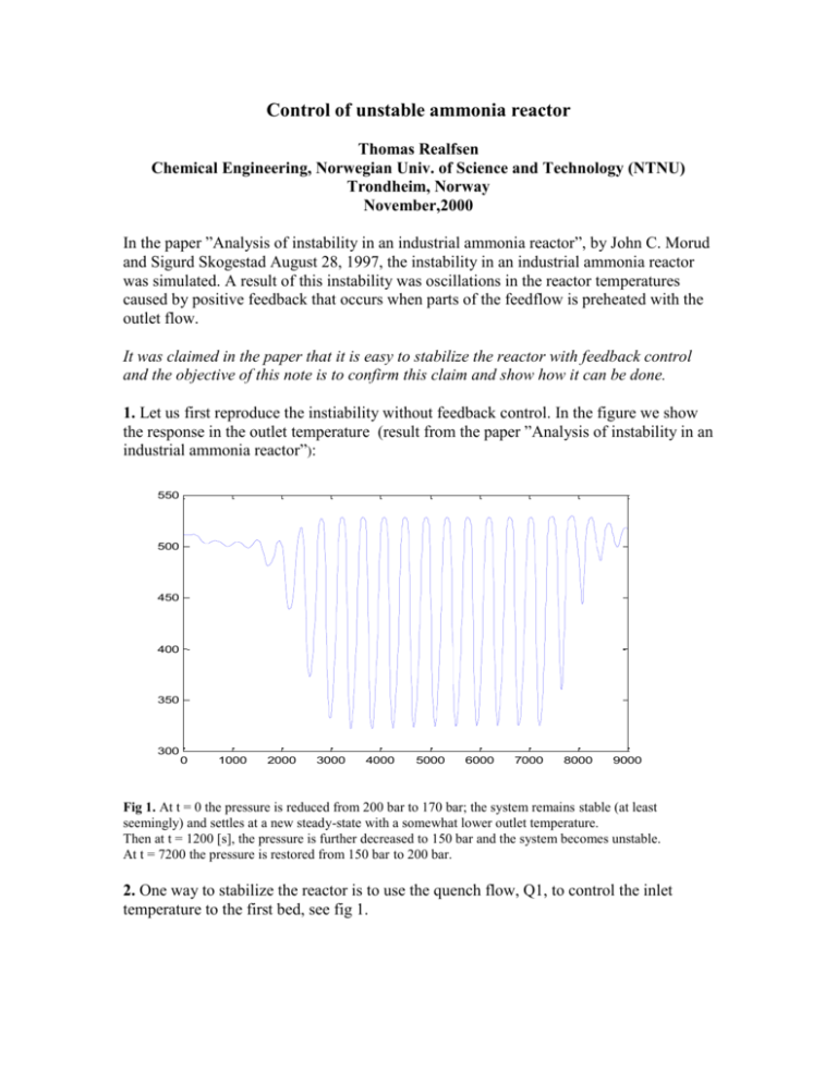
1. Let us first reproduce the instiability without feedback control. In the figure we show
the response in the outlet temperature (result from the paper ”Analysis of instability in an
industrial ammonia reactor”):
550
500
450
400
350
300
0
1000
2000
3000
4000
5000
6000
7000
8000
9000
Fig 1. At t = 0 the pressure is reduced from 200 bar to 170 bar; the system remains stable (at least
seemingly) and settles at a new steady-state with a somewhat lower outlet temperature.
Then at t = 1200 [s], the pressure is further decreased to 150 bar and the system becomes unstable.
At t = 7200 the pressure is restored from 150 bar to 200 bar.
2. One way to stabilize the reactor is to use the quench flow, Q1, to control the inlet
temperature to the first bed, see fig 1.
Fig 2. Ammonia reactor with feedback control
Simulation of the pressure reduction using this feedback structure with simple
proportional control shows that we have a stable system:
515
510
505
500
495
490
0
1000
2000
3000
4000
5000
6000
7000
8000
9000
Fig3. Feedback control of inlet temperature . At t = 0 the pressure is reduced from 200 bar to 170 bar; and
then at t = 1200 [s] the pressure is further decreased to 150 bar . The system remains stable!
At t = 7200 the pressure is restored from 150 bar to 200 bar.
3. Now try another simulation (with feedback) where at t = 1200 [s] the pressure is
reduced from 200 bar to 150 bar. Again the system remains stable:
512
510
508
506
504
502
500
498
496
494
492
0
1000
2000
3000
4000
5000
6000
7000
8000
9000
Fig4. The outlet temperature stabilized at a new lower steady-state.
How to produce the results in figure 1,2,3 and 4:
Go to subdirectory control and see matlab files reguleringsim.m and concprof.m (the files
are also listed below)
.
-To reproduce the unstability in figure 1, the percentage signs in front of section 1 must
be deleted (let the percentage signs in front of section 2 and 3 remain).
-To reproduce the results from figure 3, the percentage signs in front of section 1 and 3
must be deleted (the percentage signs in section 2 must remain).
-To reproduce figure 4, the percentage signs before section 2 and 3 must be deleted (the
percentage signs in section 1 must remain).
To reproduce the results made in this paper it’s enough to make the changes in the matlab
file reguleringsim. The product concentration can also be produced, the changes above
must then also be made in the matlab file concprof (it’s done this way to prevent that the
concentration plot follows the iterations made in the ode-solver).
APPENDIX: FILES
main.m
clear all
startup
fcorr=0.5; epsnr=1.e-4;
%problems (fcorr=0.5)
% decrease fcorr if convergense
Tinit=linspace(360,510,30);
%To = 511.565
% gives upper steady-state ;
Tss1=ssnr(Tinit,fcorr,epsnr); % steady-state vector
t_start=0;
t_end=9000;
tspan=[t_start t_end];
[tid,T]=ode15s('reguleringsim',tspan,Tss1);
%%%%%%%%%%%%%%%%%%%%%%%%%%%%%%%%%%%%%%
Cvec=[];
for i=length(tid):-1:1
c=concprof(tid(i),T(i,:)');
Cvec(i,:)=c(:)';
end
%%%%%%%%%%%%%%%%%%%%%%%%%%%%%%%%%%%%%%%
figure(1)
plot(tid,T(:,1))
figure(2)
plot(tid,T(:,30))
figure(3)
plot(tid,Cvec(:,30))
reguleringsim.m
function Tprime=reguleringsim(t,T)
global mc mh Cp Cpc Q1 Q2 Q3 Npoint Tf cf dm1 dm2 dm3 dHrx
u conc p
% comment: For simplicity we use rx((T(i),c(i-1)) rather
%than rx((T(i),c(i))
%section1.--Reconstruction of unstable ammonia reactor----%
if t<1200
p=170;
elseif (t>=1200 & t<=7200)
p=150;
else t>7200
p=200;
end;
%---------------------------------------------------------%
%section2.--New steady-state------------------------------%
%if t>1200
%
p=150;
%else
%
p=200;
%end;
%---------------------------------------------------------%
%section3.--P-controller----------------------------------%
%Kc=3;
%Q1=16.11+Kc*(T(1)-369.4); % positiv feedback, e=y-r
%mc=mh-(Q1+Q2+Q3);
%---------------------------------------------------------%
m1=mc+Q1;
m2=m1+Q2;
m3=m2+Q3;
% Conc. in bed 1:
c(1)=cf+dm1*rx(T(1),cf)/m1;
for i=2:10
c(i)=c(i-1)+dm1*rx(T(i),c(i-1))/m1;
end
% Quench 2:
cin2=m1/m2*c(10)+Q2/m2*cf;
% Conc. in bed 2
c(11)=cin2+dm2*rx(T(11),cin2)/m2;
for i=12:20
c(i)=c(i-1)+dm2*rx(T(i),c(i-1))/m2;
end
% Quench 3:
cin3=m2/m3*c(20)+Q3/m3*cf;
% Conc. in bed 3
c(21)=cin3+dm3*rx(T(21),cin3)/m3;
for i=22:30
c(i)=c(i-1)+dm3*rx(T(i),c(i-1))/m3;
end
%%%%%%%%%%%%%%%%%%%%%%%%%%%%%%%%%%%%%%%%%%%%%%%%
% Quench 1:
Ti=hx(T(30),Tf); Tin1=mc/m1*Ti+Q1/m1*Tf;
% dTdt in bed 1:
dTdt(1)=(m1*Cp*(Tin1-T(1))+dm1*rx(T(1),cf)*dHrx)/(dm1*Cpc);
for i=2:10
dTdt(i)=(m1*Cp*(T(i-1)-T(i))+dm1*rx(T(i),c(i1))*dHrx)/(dm1*Cpc);
end
% Quench 2:
Tin2=m1/m2*T(10)+Q2/m2*Tf;
% dTdt in bed 2:
dTdt(11)=(m2*Cp*(Tin2T(11))+dm2*rx(T(11),cin2)*dHrx)/(dm2*Cpc);
for i=12:20
dTdt(i)=(m2*Cp*(T(i-1)-T(i))+dm2*rx(T(i),c(i1))*dHrx)/(dm2*Cpc);
end
% Quench 3:
Tin3=m2/m3*T(20)+Q3/m3*Tf;
% dTdt in bed 3:
dTdt(21)=(m3*Cp*(Tin3T(21))+dm3*rx(T(21),cin3)*dHrx)/(dm3*Cpc);
for i=22:30
dTdt(i)=(m3*Cp*(T(i-1)-T(i))+dm3*rx(T(i),c(i1))*dHrx)/(dm3*Cpc);
end
Tprime=dTdt;
conc=c;
Tprime=Tprime';
concprof.m
% This function are used only for plotting concentration
%out of reactor
function c=concprof(t,T)
global mc mh Cp Cpc Q1 Q2 Q3 Npoint Tf cf dm1 dm2 dm3 dHrx
u conc p
% comment: For simplicity we use rx((T(i),c(i-1)) rather
%than rx((T(i),c(i))
%section1.--Reconstruction of unstable ammonia reactor----%
if t<1200
p=170;
elseif (t>=1200 & t<=7200)
p=150;
else t>7200
p=200;
end;
%---------------------------------------------------------%
%section2.--New steady-state------------------------------%
%if t>1200
%
p=150;
%else
%
p=200;
%end;
%---------------------------------------------------------%
%section3.--P-controller----------------------------------%
%Kc=3;
%Q1=16.11+Kc*(T(1)-369.4); % positiv feedback, e=y-r
%mc=mh-(Q1+Q2+Q3);
%---------------------------------------------------------%
m1=mc+Q1;
m2=m1+Q2;
m3=m2+Q3;
% Conc. in bed 1:
c(1)=cf+dm1*rx(T(1),cf)/m1;
for i=2:10
c(i)=c(i-1)+dm1*rx(T(i),c(i-1))/m1;
end
% Quench 2:
cin2=m1/m2*c(10)+Q2/m2*cf;
% Conc. in bed 2
c(11)=cin2+dm2*rx(T(11),cin2)/m2;
for i=12:20
c(i)=c(i-1)+dm2*rx(T(i),c(i-1))/m2;
end
% Quench 3:
cin3=m2/m3*c(20)+Q3/m3*cf;
% Conc. in bed 3
c(21)=cin3+dm3*rx(T(21),cin3)/m3;
for i=22:30
c(i)=c(i-1)+dm3*rx(T(i),c(i-1))/m3;
end