2006-04-19
BIOSTAT 2015
Statistical Foundations for Bioinformatics Data Mining
Target readings: Hastie, Tibshirani, Friedman,
Section 4.5 Separating Hyperplanes (with many misprints in older editions),
and Chapter 12 Support Vector Machines
Separating hyperplanes
 Not unique.
 May not exist.
Fig. 4.13.
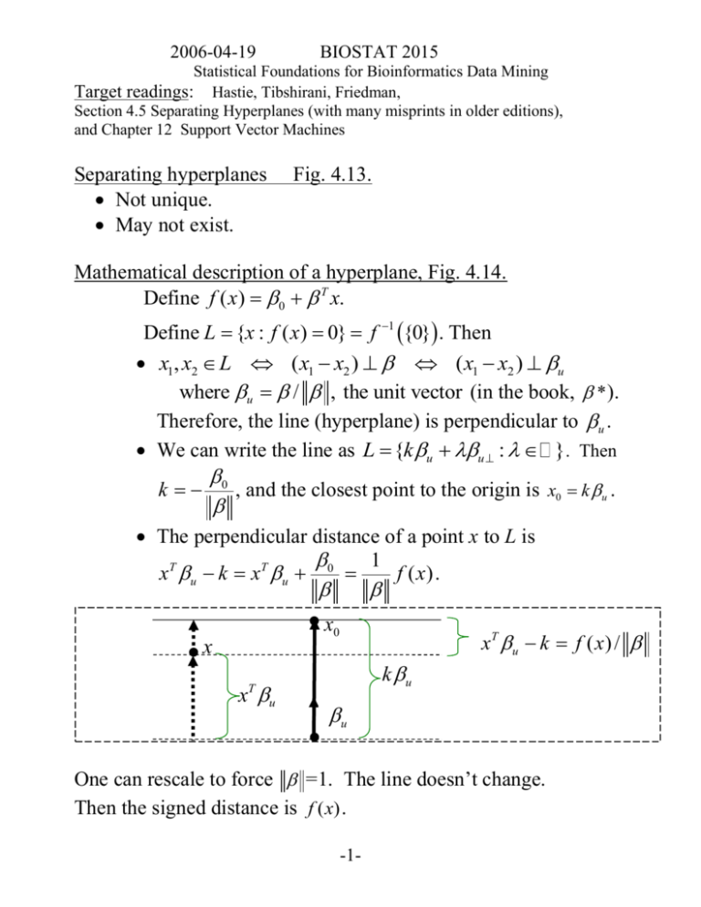
Mathematical description of a hyperplane, Fig. 4.14.
Define f ( x)   0   T x.
Define L  {x : f ( x)  0}  f 1 {0}. Then
 x1, x2  L  ( x1  x2 )    ( x1  x2 )  u
where u   /  , the unit vector (in the book,  * ).
Therefore, the line (hyperplane) is perpendicular to  u .
 We can write the line as L  {k u  u  :   }. Then
k 
0
, and the closest point to the origin is x0  k u .

 The perpendicular distance of a point x to L is

1
xT  u  k  xT  u  0 
f ( x) .


x0
xT  u  k  f ( x ) / 
x
x u
k u
T
u
One can rescale to force  =1. The line doesn’t change.
Then the signed distance is f ( x) .
-1-
2006-04-19
BIOSTAT 2015
Statistical Foundations for Bioinformatics Data Mining
Rosenblatt’s perceptron learning algorithm:
Goal: minimize over  , 0 the exponential loss
 min(0,
i
 yi f ( xi ))   | yi f ( xi ) | I {sign( f ( xi ))  yi } 
i

iMisclassified
| yi f ( xi ) |
where yi {1,1}. See Fig 4.15.
Strategy: gradient descent, one observation at a time.
that is,       yi xi  .
 0 
 yi 
This converges to a separating hyperplane if one exists, but
 Not unique
 May take a very long time to converge
 If no s.h. exists, failure to converge may be tough to detect.
 The learning rate  -- what should it be?
 
 D /  



   
 D /  
0
 0  0

Support vector classifiers: see Fig 12.1.
To get a unique separating hyperplane, maximize the margin,
C , yi yˆi  yi ( xiT   0 )  C, i  1,..., n which is half the width of
the separating strip. Because the scale is arbitrary in the definition
of f, restrict  to be of unit length.
Equivalently,
minimize  subject to perfect classification with margin C:
yi yˆi  yi ( xiT   0 )  1, i  1,..., n
1
yi  xiT u  k  
, i  1,..., n
i.e.

1
so that C 
.

The points for which yi ( xiT   0 )  1 are the support points.
-2-
2006-04-19
BIOSTAT 2015
Statistical Foundations for Bioinformatics Data Mining
Modification when no S.H. exists: Fig 12.1
Define slack variables 1,..,  N . Maximize C subject to

yi ( xiT    0 )  C (1  i ), i  1,..., n,
i
K
Misclassification is equivalent to i  1, so K is the max acceptable
number of misclassifications. Again, we convert the goal from
maximizing C to minimizing  , subject to
all yi ( xiT    0 )  1  i , all i  0,

i
 K.
Note: “robustness” to points far from the boundary (unlike linear
discriminant analysis). See Fig. 12.2 for an example.
Algorithm:
1
2
    i subject to
2
all yi ( xiT   0 )  1  i , all i  0 .”
for a fixed smoothing parameter 
(in a sense, boundng the #training set misclassifications).
A) Reformulate as: “minimize
B) Set up the Lagrangian
1
2
LP      i    i  yi ( xiT    0 )  (1  i )   ii ,
2
set the derivatives w.r.t.  ,  0,{i } , and solve for  ,  0,{i } in
terms of the Lagrange multipliers { } .
-3-
2006-04-19
BIOSTAT 2015
Statistical Foundations for Bioinformatics Data Mining
C) Substitute into LP to get the “dual”
1
LD   i   i i ' yi yi ' xiT xi '
2 i ,i '
and maximize it w.r.t.  ’s, but subject to “Karush-Kuhn-Tucker
conditions”: “quadratic programming with linear constraints”:
 i  yi ( xiT    0 )  (1  i )  0
ii  0
yi ( xiT    0 )  (1  i )  0
Because LP /   0      i yi xi , the estimated f is a
linear combination of inner products (  x, xi  xT xi ):
f ( x)  xT      xT  i yi xi   
  i yi  x, xi    
Support Vector Machines
Use an old trick: expand the set of features with derived
covariates h( x) .
f ( x)  h( x)T      h( x)T  i yi h( xi )   
  i yi  h( x), h( xi )    
Simpler: skip defining the h’s, just define the kernel function
K ( x, x ')  h( x), h( x ')  .
Then
-4-
2006-04-19
BIOSTAT 2015
Statistical Foundations for Bioinformatics Data Mining
f ( x)    i yi K ( x, xi )   
Examples:
dth degree polynomial:
K ( x, x ')  (1  xT x ') 2
Radial basis:
K ( x, x ')  exp( x  x ' / c)
Neural network :
K ( x, x ')  tanh(k1xT x ' k2 )
2
See Fig. 12.3 for our standard example, using a radial basis, where
the fit is greatly improved.
For the 2nd degree polynomial for two features, we have
K ( X , X ')  (1  X , X ' ) 2  (1  X 1 X 1 ' X 2 X 2 ') 2
 1  2 X1 X1 ' 2 X 2 X 2 ' ( X1 X 1 ') 2  ( X 2 X 2 ') 2  2 X 1 X 1 ' X 2 X 2 '
So the df is M=6, and in essence we are using derived features
h( x1 , x2 )  (1, 2 x1 , 2 x2 , x12 , x22 , 2 x1 x2 )
which give K ( x, x ')  h( x), h( x ')  .
Then the solution is of the form
N
fˆ ( x)  ˆi yi K ( x, xi )  0 .
i 1
This looks like a fit with df = N + 1, but it’s actually 7.
-5-
2006-04-19
BIOSTAT 2015
Statistical Foundations for Bioinformatics Data Mining
SVM as a Penalization Method
It turns out that solving the SVM problem is equivalent to
N
1  y f ( x )

min
 
0,
i 1
i
i
 

2
where the subscript “+” means “positive part” (min with 0).
The relationship between smoothing parameters is   1/(2 ) .
See Fig. 12.4 p.380 for the relationship between various loss
functions. Compare with figure 10.4 (p.309).
See Table 12.1 for the relationship among the population
minimizers (if you knew the model exactly, what would your
decision be?) Recall that (-)Bin Log-lik and Exponential loss have
the same minimizer f ( X )  log( p /(1  p)), p  Pr(Y  1| X ) .
Loss
function
(-1)
Binomial
log
likelihood
Squared
error
SVM
L(Y , f ( X ))
log(1  e Yf ( X ) )
Minimizing function
f ( X )  log
Pr(Y  1| X )
Pr(Y  1| X )
(Y  f ( X )) 2
f ( X )  Pr(Y  1| X )  Pr(Y  1| X )
[1  Yf ( X )]
1 if Pr(Y  1| X )  Pr(Y  1| X )
f (X )  
1 if Pr(Y  1| X )  Pr(Y  1| X )
-6-
2006-04-19
BIOSTAT 2015
Statistical Foundations for Bioinformatics Data Mining
Reproducing Kernel Hilbert Spaces
The basis functions h may be derived from an eigen-expansion in
function space:

K ( x, x ')   m ( x)m '( x) m
m1
with hm ( x)   m m ( x) . Then
N
min 1  yi f ( xi )  
0 ,

2
i 1
for f ( x)   x  0 essentially becomes
T
N
1  y f ( x )

min
 
0,
i 1
i
i
T


K

where K is the N by N matrix of evaluations on pairs of training features.
This set-up applies also to our smoothing splines model.
-7-