SUPPLEMENTARY APPENDIX B
Condition for evolutionary stability
Derivation of the marginal value argument
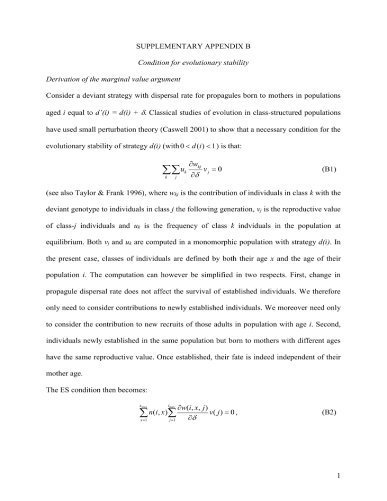
Consider a deviant strategy with dispersal rate for propagules born to mothers in populations
aged i equal to d’(i) = d(i) + . Classical studies of evolution in class-structured populations
have used small perturbation theory (Caswell 2001) to show that a necessary condition for the
evolutionary stability of strategy d(i) (with 0  d (i )  1 ) is that:
 u
k
k
j
wkj

vj  0
(B1)
(see also Taylor & Frank 1996), where wkj is the contribution of individuals in class k with the
deviant genotype to individuals in class j the following generation, vj is the reproductive value
of class-j individuals and uk is the frequency of class k indviduals in the population at
equilibrium. Both vj and uk are computed in a monomorphic population with strategy d(i). In
the present case, classes of individuals are defined by both their age x and the age of their
population i. The computation can however be simplified in two respects. First, change in
propagule dispersal rate does not affect the survival of established individuals. We therefore
only need to consider contributions to newly established individuals. We moreover need only
to consider the contribution to new recruits of those adults in population with age i. Second,
individuals newly established in the same population but born to mothers with different ages
have the same reproductive value. Once established, their fate is indeed independent of their
mother age.
The ES condition then becomes:
xmax
w(i, x, j )
v( j )  0 ,

j 1
imax
 n (i , x ) 
x 1
(B2)
1
where v(j) is the reproductive value of a new recruit in a population of age j, and w(i,x,j) the
contribution of an individual of age x reproducing in a population of age i to new recruits in a
population of age j the following year. Those contributions are:
if j  i  1 then w(i, x, j )  (1  c)V j g ( j  1) f ( x )d '(i )
(B3)
if j  i  1 then w(i, x, i  1)  1  e(i)  g (i) f ( x) 1  d '(i)  (1  c)Vid '(i) 
(B4)
By taking derivatives and using equation (B2) we obtain the necessary condition for
evolutionary stability of d(i) as in equations (3c) and (4). Conditions for evolutionary stability
at limit feasible values for the dispersal rate (0 or 1) can similarly be derived as in equations
(3a) and (3b).
Computation of reproductive values
We define the matrix B={bij}, which elements are the lifetime contribution of an individual
recruited in a population of age j to new recruits in population of age i:
xmax
bij  
x 1
L( j  x  1)
l ( x ) w0 ( j  x  1, x, i ) ,
L( j )
(B5)
where w0(j,x,i) is w(j,x,i) evaluated at =0. The individual reproductive values v={v(i)} of
new recruits established in the different population types are obtained as the left-eigenvector
of matrix B.
2