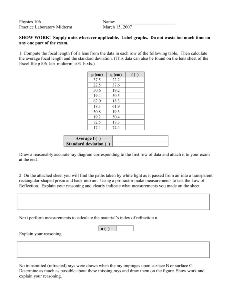
Physics 106
Practice Laboratory Midterm
Name: __________________________
March 15, 2007
SHOW WORK! Supply units wherever applicable. Label graphs. Do not waste too much time on
any one part of the exam.
1. Compute the focal length f of a lens from the data in each row of the following table. Then calculate
the average focal length and the standard deviation. (This data can also be found on the lens sheet of the
Excel file p106_lab_midterm_s03_b.xls.)
p (cm)
37.5
22.5
50.6
19.4
62.0
18.3
50.8
19.2
72.5
17.4
q (cm)
22.2
37.6
19.2
50.5
18.3
61.9
19.3
50.4
17.3
72.4
f( )
Average f ( )
Standard deviation ( )
Draw a reasonably accurate ray diagram corresponding to the first row of data and attach it to your exam
at the end.
2. On the attached sheet you will find the paths taken by white light as it passed from air into a transparent
rectangular-shaped prism and back into air. Using a protractor make measurements to test the Law of
Reflection. Explain your reasoning and clearly indicate what measurements you made on the sheet.
Next perform measurements to calculate the material’s index of refraction n.
n( )
Explain your reasoning.
No transmitted (refracted) rays were drawn when the ray impinges upon surface B or surface C.
Determine as much as possible about these missing rays and draw them on the figure. Show work and
explain your reasoning.
3. A plunger tube has resonances at the following lengths. Determine the frequency of the sound that is
driving the tube.
Length (cm)
7.2
25.1
43.2
60.7
Explain your reasoning.
Fit the envelope function for the data found on the beat sheet of the Excel file
p106_lab_midterm_s03_a.xls to the formula
y(t) = yeq + A cos( 2  t / T + )
Title it Beat Data (Smith) with your last name in place of Smith. Print it out. (Make sure the graph is
highlighted when you print so that you do not print the data.) Enter your fit parameters into the following
table.
yeq ( )
A( )
T( )
( )
The beat data above was obtained by having two distinct driving frequencies. The lower was 350 Hz.
Estimate the higher frequency.
Other frequency ( )
Explain your reasoning.
4. Standing wave patterns were observed at the following frequencies. The corresponding node-to-node
distances were measured. Calculate the velocity for each row of data. (This data can also be found on the
standing wave sheet of the Excel file p106_lab_midterm_s03_b.xls.)
Frequency
(Hz)
12
20
28
36
Node-to-node
distance (cm)
112
69
50
37
Velocity ( )
Plot the node-to-node distance versus frequency and fit it to a power law. Title it Standing Wave Data
(Smith). Compare your fit to what you should expect theoretically.
There were some knots toward the end of the cord that were not untied when its length was measured.
What effect would this have on the (F/)1/2 prediction of velocity? Explain.
5. The amplitude (maximum angle) of a pendulum was varied, and the period was measured. The
resulting data follows. (This data can also be found on the pendulum sheet of the Excel file
p106_lab_midterm_s03_b.xls.)
Maximum
Angle M
(degrees)
5
10
15
20
25
30
35
40
45
50
55
60
65
70
75
Maximum
Angle M
(radians)
Sin(M/2)
Period (s)
0.800442
0.801534
0.803516
0.80618
0.809699
0.81398
0.819018
0.824991
0.831726
0.839315
0.847794
0.857044
0.867117
0.878072
0.889636
Fill in the missing columns. Note that third column is sin(M/2) NOT sin(M). Then plot the period
versus Sin(M/2) and fit it to a polynomial of order two. Entitle it “Smith: Pendulum Data.” According
to theory what should the coefficient of the square term be?
You want a pendulum that has a period of 1.85 s determine the necessary mass, mass and amplitude and
enter them into the table below.
Mass ( )
Length ( )
Amplitude ( )
6. A mass was hung vertically from a spring. The position versus time data was taken for several masses
and fit to the form
 2

y (t )  yeq  A cos
t  0  ,
 T

resulting in the following fit parameters
Hanger +
Mass (g)
50
100
150
200
250
yeq (m)
A (m)
T (s)
0
.692
.666
.645
.617
.593
0.0263
0.0256
0.0281
0.0335
0.0289
0.52
0.60
0.69
0.76
0.82
5.8
5.8
3.2
2.3
3.8
Determine the spring’s force constant graphically. Title it Spring Data (Smith) with your last name in
place of Smith. Print it out. (Make sure the graph is highlighted when you print so that you do not print
the data.)
Spring’s force constant ( )
Suppose the 250-g mass above had been pulled down further before being released. Categorize the
parameters as “will change”, “might change” or “won’t change” (within experimental error) and explain
your choice.
Parameter Will change,
Might change or
Won’t change
yeq
A
T

Explanation