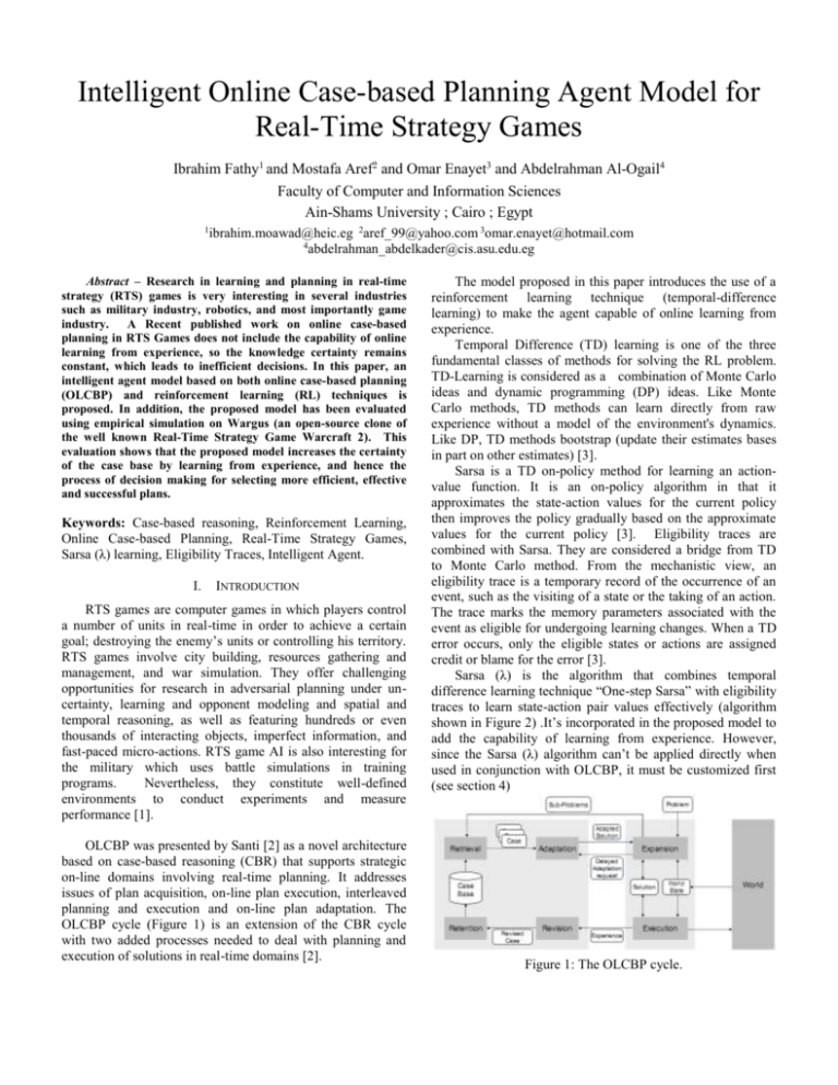
Intelligent Online Case-based Planning Agent Model for
Real-Time Strategy Games
Ibrahim Fathy1 and Mostafa Aref2 and Omar Enayet3 and Abdelrahman Al-Ogail4
Faculty of Computer and Information Sciences
Ain-Shams University ; Cairo ; Egypt
1
ibrahim.moawad@heic.eg 2aref_99@yahoo.com 3omar.enayet@hotmail.com
4
abdelrahman_abdelkader@cis.asu.edu.eg
Abstract – Research in learning and planning in real-time
strategy (RTS) games is very interesting in several industries
such as military industry, robotics, and most importantly game
industry. A Recent published work on online case-based
planning in RTS Games does not include the capability of online
learning from experience, so the knowledge certainty remains
constant, which leads to inefficient decisions. In this paper, an
intelligent agent model based on both online case-based planning
(OLCBP) and reinforcement learning (RL) techniques is
proposed. In addition, the proposed model has been evaluated
using empirical simulation on Wargus (an open-source clone of
the well known Real-Time Strategy Game Warcraft 2). This
evaluation shows that the proposed model increases the certainty
of the case base by learning from experience, and hence the
process of decision making for selecting more efficient, effective
and successful plans.
Keywords: Case-based reasoning, Reinforcement Learning,
Online Case-based Planning, Real-Time Strategy Games,
Sarsa (λ) learning, Eligibility Traces, Intelligent Agent.
I.
INTRODUCTION
RTS games are computer games in which players control
a number of units in real-time in order to achieve a certain
goal; destroying the enemy’s units or controlling his territory.
RTS games involve city building, resources gathering and
management, and war simulation. They offer challenging
opportunities for research in adversarial planning under uncertainty, learning and opponent modeling and spatial and
temporal reasoning, as well as featuring hundreds or even
thousands of interacting objects, imperfect information, and
fast-paced micro-actions. RTS game AI is also interesting for
the military which uses battle simulations in training
programs.
Nevertheless, they constitute well-defined
environments to conduct experiments and measure
performance [1].
OLCBP was presented by Santi [2] as a novel architecture
based on case-based reasoning (CBR) that supports strategic
on-line domains involving real-time planning. It addresses
issues of plan acquisition, on-line plan execution, interleaved
planning and execution and on-line plan adaptation. The
OLCBP cycle (Figure 1) is an extension of the CBR cycle
with two added processes needed to deal with planning and
execution of solutions in real-time domains [2].
The model proposed in this paper introduces the use of a
reinforcement learning technique (temporal-difference
learning) to make the agent capable of online learning from
experience.
Temporal Difference (TD) learning is one of the three
fundamental classes of methods for solving the RL problem.
TD-Learning is considered as a combination of Monte Carlo
ideas and dynamic programming (DP) ideas. Like Monte
Carlo methods, TD methods can learn directly from raw
experience without a model of the environment's dynamics.
Like DP, TD methods bootstrap (update their estimates bases
in part on other estimates) [3].
Sarsa is a TD on-policy method for learning an actionvalue function. It is an on-policy algorithm in that it
approximates the state-action values for the current policy
then improves the policy gradually based on the approximate
values for the current policy [3]. Eligibility traces are
combined with Sarsa. They are considered a bridge from TD
to Monte Carlo method. From the mechanistic view, an
eligibility trace is a temporary record of the occurrence of an
event, such as the visiting of a state or the taking of an action.
The trace marks the memory parameters associated with the
event as eligible for undergoing learning changes. When a TD
error occurs, only the eligible states or actions are assigned
credit or blame for the error [3].
Sarsa (λ) is the algorithm that combines temporal
difference learning technique “One-step Sarsa” with eligibility
traces to learn state-action pair values effectively (algorithm
shown in Figure 2) .It’s incorporated in the proposed model to
add the capability of learning from experience. However,
since the Sarsa (λ) algorithm can’t be applied directly when
used in conjunction with OLCBP, it must be customized first
(see section 4)
Figure 1: The OLCBP cycle.
The next section gives a brief background about related
work based on OLCBP and hybrid CBR/RL techniques.
Section 3 describes the general architecture of the proposed
intelligent case-based planning agent model. Section 4
explains how OLCBP and RL using Sarsa (λ) are hybridized.
Section 5 evaluates the proposed model by applying empirical
simulation on Wargus game. Finally, section 6 concludes the
work presented in this paper and presents new ideas for future
work.
Using case-based reasoning in support of reinforcement
learning or vice versa is not a novel idea. Sharma [5]
presented a multi-layered architecture named CARL (Casebased Reinforcement Learner) for achieving transfer learning
using a hybrid CBR/RL approach and applied it to RTS
games. CARL uses the RL algorithm, Q-Learning, in order to
revise the cases. CARL, however; doesn’t support many
features that are found in Darmok such as case acquisition,
case adaptation … etc. Johansen [6] presented another
CBR/RL system for learning micro-management in RTS
games, however; it doesn’t target high level planning.
Molineaux [7] presented an RL/CBR algorithm to learn
continuous action models for selecting actions in RTS Games.
Apart from RTS Games, Gabel [8] used CBR for function
approximation. Finally, Bianchi [9] improved RL using casebased heuristics.
The work presented in this paper is based on Darmok [2]
with the addition of the capability of learning from experience
and evaluating cases using the Sarsa (λ) RL algorithm. This
evaluation let the system choose not only the most suitable
plan for the current game state, but also the most efficient one.
Figure 2: The original Sarsa (λ) algorithm.
II. BACKGROUND
Online case-based planning was implemented in the
Darmok system [2]. Darmok solves the case acquisition
problem by observing how human play with the support of
human annotations. Darmok also, interleaves planning and
execution on-line in order to achieve efficient on-line planning
that is reactive to the current situation. It introduces the idea of
delayed plan adaptation in order to insure its validity for the
current time if the plan was retrieved earlier. Finally, Darmok
implements plan adaptation techniques that are efficient to be
executed on-line.
III. INTELLIGENT OLCBP AGENT MODEL
In this paper, a new AI agent model capable of online
planning with online learning is introduced. The agent model
architecture is considered as an evolution of the Darmok
system [2] by adding the capability of learning from
experience. As shown in Figure 5, the architecture consists of
two main phases: an offline learning phase, and an online
planning and learning phase.
The offline learning phase –which is not our interest in
this paper - is based on Santiago’s [4] work and is used to
populate the cases in case base.
Santiago [4] presented a set of algorithms that can be used
to -automatically- learn plans from human demonstrations and
thus an automatic approach for case acquisition. During case
acquisition, the system starts to learn plans by observing game
play and strategies between two different opponents (i.e.
human and computer) and then, deduces and forms several
cases. The system receives raw traces that form the game
played by the human. Using Goal Matrix Generation, these
traces are converted into raw plan. Further, a Dependency
Graph is constructed for each raw plan, which lets the system
be aware of the following points: 1) The dependencies between the raw plan steps.
2) Which plan steps are suitable to be executed in
parallel?
Next, a Hierarchal Composition for each raw plan is formed
in order to shrink raw plan size and substitute group of related
steps with the goal step. Finally, all the learnt plans are
retained in the case base.
Figure 3: Case representation.
Each case is composed of 8 components (shown in Figure 3)
1. Goal: the goal that is achieved by the case plan.
2. Situation: where the case can be applied.
3. Shallow Features: set of sensed features from the
environment which requires low computation overhead.
4. Deep Features: set of sensed features from the
environment which requires high computation overhead.
5. Certainty Factor: a decimal that indicates the certainty of
success when applying its case. Negative certainty factor
means uncertain, while positive means certain. Its value
constitutes the magnitude of certainty.
6. Eligibility Trace: a decimal that represents the
responsibility (eligibility) of the case for reaching the
current state.
7. Prior Confidence: a decimal, ranges between zero and
one, set by an expert, indicating the confidence of success
when using that case from the expert’s point of view.
8. Behavior: coins the actual plan to be used
After the agent learns cases that serve as basic ingredients
for playing the game [4], it then set to be ready to play against
different opponents. The phase where the agent plays against
opponents is called online planning and learning phase (i.e.
online phase). The planning comes from expansion and
execution of current plan whereas learning comes from the
revision of the applied plans. The online planning and
learning phase consists of expansion, execution, retrieval,
adaptation, reviser, and current plan components.
As shown in Figure 3, a behaviour consists of:
preconditions that must be satisfied before the plan execution,
alive conditions that must be satisfied while the plan is being
executed, success conditions that must be satisfied after the
plan has been executed, and snippet that is a set of the plan
steps, where each plan step consists of a set of parallel
actions/goals.
The Expansion module expands ready open goals in the
current plan. The Readiness means that all snippets before that
goal were executed successfully while Opening means that
this goal has no assigned behaviour.
The Retrieval module selects the most efficient plan using:
situation assessment to get most suitable plan, E-Greedy
selection policy to determine whether to explore or exploit.
Equation 1 in figure 4 shows the exploration/exploitation
equation. In exploitation, the predicted performance of all
cases is computed and the best case is selected using equation
2 of Figure 4. In exploration, a random case is selected.
The situation assessment module is built through
capturing most representative shallow features of the
environment, building Situation-Model that maps set of
shallow features to situation, building Situation-Case Model to
classify each case for specific situation, and building
Situation-Deep Feature Model to provide set of deep features
that are important for predicted situation.
The selected behaviour is passed to the Adaptation
module to adapt the plan for the current situation. Adaptation
means removal of unnecessary actions in the plan and then
adding the satisfied actions.
Figure 4: Retrieval process equations.
Execution module starts to execute plan actions whenever
their preconditions are satisfied. To execute plans, the
execution module starts to search for ready snippets, and then
sends these ready snippets for execution (to the game),
updates the current status of executing snippets whether
succeeded or failed and finally, updates status of executing
actions from each snippet.
After a complete snippet execution, the reviser module
starts its mission. The importance of revision originated from
the fact that interactive and intelligent agents must get
feedback from the environment to improve their performance.
The learnt plans were based on an expert’s actions which are
not necessarily the best actions. The reviser adjusts the case
performance according to Temporal Difference learning with
Sarsa (λ) Online Policy Learning Algorithm. Finally, the
adjusted plan is retained in the case base using the retainer
module.
Figure 5: Intelligent OLCBP agent model.
3) It retrieves all cases with a similar S (Goal and
Situation) to the S of the retrieved case Cr and stores
the result in E.
IV. HYBRID OLCBP/RL ALGORITHM USING SARSA(λ)
The approach presented in this paper hybridizes Online Casebased Planning (OLCBP) and Reinforcement Learning (RL)
using a proposed new version of Sarsa (λ) algorithm (shown in
Figure 6). In order to show how Sarsa (λ) algorithm has been
customized, Table 1 maps the old symbols\meanings in the
original Sarsa (λ) algorithm (shown in Figure 2) to the new
symbols\meanings used in this work.
4) It updates the eligibility of all cases in E according to
the following equation:
e (C) = γ λ e (C)
Where: λ is the trace decay parameter, which controls
the rate of decay of the eligibility trace of all cases.
As it increases, the cases preserve most of their
eligibility and thus are affected more with any
rewards or punishments.
Every time the agent retrieves a case to satisfy a certain goal,
the agent –in RL terms- is considered to have a new state, and
starts the applying the algorithm, which goes through the
following steps:
Notice that only cases with similar goal and situation
have their eligibility updated, since cases with similar
goal and situation are considered to constitute a pool
of states (in RL terms) that need to take the
responsibility of choosing the current case and thus
have their eligibilities updated.
1) It increments the eligibility of the retrieved case
according to the following equation:
e (Cr) = e (Cr) + 1
Where: Cr is the retrieved case.
However, the performance of the entire case base is
updated (mainly the used cases only, as unused cases
will have an eligibility of zero and thus doesn’t
change in value), because different types of cases
affect each other’s performance, for example, a case
achieving the “Build Army” goal will certainly affect
the performance of the next used case which achieves
the “Attack” goal.
2) It then updates the certainty factors of all cases in its
case base according to the following equation:
Q(C) = Q(C) + α δ e(C)
Where α is the learning rate, e(C) is the eligibility of the
case C and δ is the temporal difference error that depends
on the following equation:
δ = R + r + γ Q (Cr) – Q (Cu)
Where:



R: a global reward whose value depends on the ratio
between the player’s power and the enemy’s power
(the global consequence). It ranges between -1 and 1. It
is very important for the agent to be aware of not only
the direct consequences of its actions but also the
global consequences.
r: a case-specific reward due to the success or failure of
the last used case(the direct consequence). It ranges
between -1 and 1. It is computed based on a heuristic
which determines how effective the plan was according
to the following formula :
γ Q (Cr) – Q (Cu) : The difference in certainty factor
between the retrieved case Cr (multiplied with the
discount rate γ) and the last used case Cu.
Notice that, in online case-based planning there could
be multiple last used cases executed in parallel; in this
condition the total temporal difference error relative to
all last used cases should be equal to:
δ = R + ∑in ri + γ Q (Cr) – Q (Ci)
Where n: number of last used cases
Observe failed or succeeded Case Cu
Compute R, r
Retrieve Case Cr via retrieval policy (E-greedy)
δ = R + r + γ Q (Cr) – Q (Cu)
e (Cr) = e (Cr) + 1
For each case C in the case base
Q(C) = Q(C) + α δ e(C)
Retrieve set of cases E with similar goal and situation
For each case C in E
e (C) = γ λ e (C)
Figure 6: Hybrid OLCBP/RL algorithm for case revision.
Table 1: Mapping between original and new symbols of Sarsa
(λ) algorithm.
Symbol
Original Meaning
New
Symbol
New Meaning
s
State
S
Goal and Situation
a
Action
P
Plan (Case Snippet)
(s,a)
State-action pair
(S,P) or
C
Case
Q(s,a)
Value of state-action
pair
Q(S,P)
or Q(C )
Certainty Factor of
case
r
reward
R
General Reward
α
Learning
Parameter
α
Learning
Parameter
δ
Temporal-Difference
Error
δ
TemporalDifference Error
e(s,a)
Eligibility trace for
state-action pair
e(S,P) or
e(C)
Eligibility trace for
case
γ
Discount rate
γ
Discount Rate
λ
Trace
Parameter
λ
Trace
Parameter
-
-
r
Goal-Specific
Reward
Rate
Decay
Rate
Decay
V. EXPERIMENTS AND RESULTS
In order to show the significance of extending online casebased planning with online learning using reinforcement
learning, consider the following simple test case, where the
case acquisition module (Offline Learning from human traces)
has just learned the following 4 cases (shown in table 2), and
initialized their certainty factors with a zero value.
Table 2: The experimental cases.
Case 1: BuildArmy1
Case 2: BuildArmy2
Goal: Build Army
Goal: Build Army
State: Enemy has a towers State: Enemy has a towers
defense. (identical to Case2)
defense. (identical to Case1)
Plan:
Plan:
-Train 15 footmen
-Train 2 ballista
-Train 5 Archers
-Train 6 Knights
Certainty Factor : 0
Certainty Factor : 0
Case 3 :Attack1
Case 4:Attack2
Goal: Attack
Goal: Attack
State: Enemy has a towers State: Enemy has a towers
defense, agent has 15 defense, agent has 2 ballista
footmen and 5 Archers exist
and 6 knights exist
Plan:
Plan:
-Attack with 15 footmen and
-Attack with 2 ballista and 6
-5 archers on towers defense
-knights on towers defense
Certainty Factor : 0
Certainty Factor : 0
In order to win, the Agent has to fulfill the 2 goals: “Build
Army” and “Attack” in order, by choosing one case for each
goal respectively.
Notice that, cases BuildArmy1 and BuildArmy2 share
identical game states, though they contain different plans for
achieving the same goal “Build Army”.
On the other hand, cases Attack1 and Attack2 achieve the
same goal but with different plans, and different game states
which are the same as the game states achieved after executing
BuildArmy1 and BuildArmy2 respectively. Using
BuildArmy1 will definitely force the agent to use Attack1 as
BuildArmy1 trains the necessary army that will be used in
Attack1. Similarly, using BuildArmy2 will definitely force
the agent to use Attack2.
It’s known in the game of Wargus, that using heavy units such as ballista and knights- to attack a towers defense is more
effective than using light units such as footmen and archers.
This means that it is highly preferable to use case
BuildArmy2 instead of case BuildArmy1, and use Attack2
which will definitely cause the agent to destroy more of the
enemies units and thus approach wining the game.
The experiment constitutes tracing the agent’s evaluation for
the cases (after achieving goals “Build Army” then “Attack”
in order) for 40 successive times. The initial empirical
simulation parameters were set as follows: Learning rate is
0.1, discount rate is 0.8, and decay rate is 0.5.
The exploration rate parameter of the E-Greedy policy used in
the retrieval process is set equal to 0.1 which is a relatively
low number. The reason why it is set low is because there
exists only 2 cases where one of them is the worst case, so
increasing the parameter means increasing the probability of
choosing the worst case which is not recommended.
The values of all the certainty factors and eligibilities of the
cases were initialized to zero. Table 3 shows the ranges of the
rewards gained after executing each of the 4 cases. Notice that
BuildArmy1 and BuildArmy2 are rewarded similarly
however; the rewards of Attack1 and Attack2 vary greatly
due to the different results of both.
Table 3: Rewards variations gained after executing the cases.
Case-specific reward
Global Reward
Case/Reward
From
To
From
To
BuildArmy1
0
0.2
0.2
0.3
BuildArmy2
0
0.2
0.2
0.3
Attack1
0
0.2
-0.8
-0.6
Attack2
0.1
0.2
0.4
0.6
Figure 7 shows a graph that compares the certainty factors of
the 2 cases BuildArmy1 and BuildArmy2 along with their
eligibility traces. E1 means Eligibility of BuildArmy1 and E2
means eligibility of BuildArmy2. Similarly, Figure 8
compares Attack1 and Attack2.
As shown in Figure 8, the certainty factor of case Attack2
exceeds that of case Attack1 which is perfectly natural since
case Attack2 causes the environment to provide the agent
with more rewards as it causes more damage to the enemy
(transforms the agent to a better game state). On the other
hand, the eligibility of Attack1 was slightly increased every
relatively big time interval (due to low exploration rate) when
an exploration decision (which leads to retrieving Attack1)
was made. Since Attack1 and Attack2 have different
situations, and since there are no other cases that have similar
goal and situations, their eligibility traces are never decayed in
this example.
In the end, it’s obvious that the agent has learned successfully
to evaluate each case and - through an indirect way – has
learned that it’s preferable to use BuildArmy2 instead of
BuildArmy1 in spite of the fact that both of them achieve the
same goal successfully.
This proves that the agent has learnt that building a smaller
heavy army in that situation (the existence of a towers
defense) is more preferable than building a larger light army.
Similarly, the agent can evaluate the entire case base and learn
the right choices.
V. CONCLUSION AND FUTURE WORK
Certainty factor/Eligibility
Value
Figure 7 – Tracing certainty factors and eligibility values of
BuildArmy1 and BuildArmy2 during 40 evaluations.
Figure 8 – Tracing certainty factors and eligibility values of
Attack1 and Attack2 during 40 evaluations.
In this paper, online case-based planning was hybridized with
reinforcement learning in order to introduce an intelligent
agent capable of planning and learning online using temporal
difference with eligibility traces: Sarsa (λ) algorithm. The
empirical evaluation has shown that the proposed model
increases the certainty of the case base by learning from
experience, and hence the process of decision making for
selecting more efficient, effective and successful plans.
Further, three main points can be considered as a future work
for the research presented in this paper:  Implementing a prototype based on the proposed model
in this paper.
 Developing a strategy/case base visualization tool
capable of visualizing agent’s preferred playing strategy
according to its learning history. This will help in
tracking the learning curve of the agent.
 Finally, designing and developing a multi-agent system
where agents are able to share their experiences together;
is a promising future work.
REFERENCES
The certainty factors of Attack1 and Attack2 affect those of
BuildArmy1 and BuildArmy2 dramatically. Using eligibility
traces has put the proper blame of failure and success in
Attack1 and Attack2 on BuildArmy1 and BuildArmy2
respectively. This caused the certainty factor of BuildArmy1
to drop down and that of BuildArmy2 to increase
dramatically (shown in figure 7).
Notice that the eligibility of BuildArmy1 is spiky as it
increases with each exploration then quickly decreases again
due to being decayed. On the other hand, when the eligibility
of BuildArmy1 reaches its peak, eligibility of BuildArmy2
reaches its lowest value (roughly, point (11, 0.4) in the graph
of figure 7) also due to being decayed (as it’s not being used).
The eligibilities of BuildArmy1 and BuildArmy2 - on the
contrary of Attack1 and Attack2 - are decayed because they
have a similar goal and game state so they are the reasons for
decaying each other’s eligibility.
Notice also, that the certainty factor of Attack1 increases in a
much larger rate than BuildArmy1 (although they are always
consequent); since the eligibility traces of Attack1 are never
decayed as it happens with BuildArmy1.
[1]M. Buro, “Call for AI research in RTS games”, Proceedings of the
AAAI-04 Workshop on Challenges in Game AI, 2004
[2]S. Ontañón, K. Mishra, N. Sugandh, and A. Ram, “On-line Case-based
Planning”, Computational Intelligence Journal, Volume 26, Issue 1, pp.
84-119, 2010.
[3]R. Sutton, A. Barto, “Reinforcement Learning, An Introduction”, MIT
press, 2005
[4]S. Ontañón, K. Mishra, N. Sugandh, and A. Ram, “Learning from
Demonstration and Case-Based Planning for Real-Time Strategy Games”,
Soft Computing Applications in Industry (ISBN 1434-9922 (Print) 18600808 (Online)), p. 293-310.
[5]M. Sharma, M. Homes, J. Santamaria, A. Irani, C. Isbell, and A. Ram,
“Transfer learning in Real-Time Strategy Games using hybrid CBR/RL”,
IJCAI'2007, page to appear. Morgan Kaufmann, 2007.
[6]M. Gunnerud, ”A CBR/RL system for learning micromanagement in
Real-Time Strategy Games”, Norwegian University of Science and
Technology, 2009.
[7]M. Molineaux, D. Aha, and P. Moore, “Learning Continuous Action
Models in a Real-Time Strategy Environment”, 2008
[8]T. Gabel, and M. Riedmiller, ”CBR for State Value Function
Approximation in Reinforcement Learning”, 2005.
[9]R. Bianchi, R. Ros, and R. Lopez, ”Improving Reinforcement Learning
by using Case-Based Heuristics”, 2009.