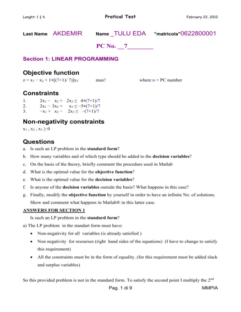
Pratical Test
Lenght: 1 ½ h
Last Name
AKDEMIR
Name _TULU
February 22, 2012
EDA
”matricola”0622800001
PC No. __7________
Section 1: LINEAR PROGRAMMING
Objective function
z = x1 − x2 + 1[(7+1)/ 7)]x3
max!
where n = PC number
Constraints
2x1 − x2 + 2x3 ≤ 4(7+1)/7
2x1 − 3x2 + x3 ≤ −5(7+1)/7
−x1 + x2 − 2x3 ≤ −(7+1)/7
1.
2.
3.
Non-negativity constraints
x1 , x2 , x3 ≥ 0
Questions
a. Is such an LP problem in the standard form?
b. How many variables and of which type should be added to the decision variables?
c. On the basis of the theory, briefly comment the procedure used in Matlab
d. What is the optimal value for the objective function?
e. What is the optimal value for the decision variables?
f. Is anyone of the decision variables outside the basis? What happens in this case?
g. Finally, modify the objective function by yourself in order to have an infinite No. of solutions.
Show and comment what happens in Matlab® in this latter case.
ANSWERS FOR SECTION 1
Is such an LP problem in the standard form?
a) The LP problem in the standart form must have:

Non-negativity for all variables (is already satisfied )

Non negativity for resourses (right hand sides of the equations) (I have to change to satisfy
this requirement)

All the constraints must be in the form of equality. (for this requirement must be added slack
and surplus variables)
So this provided problem is not in the standard form. To satisfy the second point I multiply the 2nd
Pag. 1 di 9
MMPIA
Lenght: 1 ½ h
Pratical Test
February 22, 2012
and the 3rd constraint with (-) and I get:
-2x1 + 3x2 - x3 ≥ 5(7+1)/7
x1 -x2 + 2x3 ≥ (7+1)/7
b) How many variables and of which type should be added to the decision variables?

Slack variables are the ones that are added in the equation when in the presence of “≤”
constraint and shows the used resources .From that we should have one for this problem.

Surplus variables are substracted from the equation in the presence of “≥” constraint and
shows the excess resourses. From that we have two for this problem.

Artificial variables
c) On the basis of the theory, briefly comment the procedure used in Matlab
the problem is presented in the form:
z=c1x1+c2x2+....
ar1x1+ar2x2+....<br
ak1x1+ak2x2+....>bk
Linear problems in matlab can be solved both graphical method and the simplex algorithm method.
However in the case of having more than 2 decision variables graphical method can not be
applicable and the simplex method must be used. For this problem the situation is we have 3
decision variables so I need to use simplex algorithm.
I need to introduce c,A,b,rel and type variables to the Matlab as I did below:
Then I enter the simplex2p(type,c,A,rel,b) and I obtain the first tableau:
Pag. 2 di 9
MMPIA
Lenght: 1 ½ h
Pratical Test
February 22, 2012
Here 10 columns and 6 rows are seen:
I&II&III columns show the decision variables
IV is the slack variable
V & VI are the surplus variables
VII&VIII&IX are the artificial variables.
First 3 rows shows the coefficients of the constraints
5th shows the objective function as (-z)
6th shows the artificial objective function (-w)
As a rule we must add two artificial variables for two surplus variables but matlab adds also for slack variables
due to the safety issues. We have 1 slack 2 surplus variables that’s why there are 3 artificial variables.
After we continue to the iteration on Matlab to obtain the optimum solution at the end of phase 1 we have:
Pag. 3 di 9
MMPIA
Lenght: 1 ½ h
Pratical Test
February 22, 2012
At the end of phase one, the element at the intersection of last column and the last row w=0 means
that we have a basic feasible solution.
X1=3.4286 x2=4.5714 x3=1.1429
In the case of having w>0 means that we have an empty feasible solution.
When we continue with second phase, the artificial variables and the last row (service row) are
eliminated. At the end of 2nd phase we should obtain the optimum solution for the original problem.
Pag. 4 di 9
MMPIA
Lenght: 1 ½ h
Pratical Test
February 22, 2012
d) What is the optimal value for the objective function?
Optimal value for the objective function is given by the matlab as a result of second phase.
Z=1.240816
e) What is the optimal value for the decision variables?
X1=0
X2=3.20
X3=3.88
f) Is anyone of the decision variables outside the basis? What happens in this case?
h)Finally, modify the objective function by yourself in order to have an infinite No. of solutions.
Show and comment what happens in Matlab® in this latter case.
To have an infinite number of solutions the objective function must be parallel at least to one of the
constaints .
In this problem the objective function is
z = x1 − x2 + 8/7 x3 If I change the coefficient of the x3 with 2 it becomes :
z = x1 − x2 + 2 x3 It will have the same coefficients with third constraint.Then If I implement this
revision on matlab I get:
Matlab shows me a warning window and it says that in this case I will have optimum solutions.I can
not have an unique optimum solution.
Pag. 5 di 9
MMPIA
Pratical Test
Lenght: 1 ½ h
February 22, 2012
Section 2: EMPIRICAL MODELS
===
Section 3: FINITE DIFFERENCE METHODS for PDE
ux, t 
 2 u  x, t 

t
x 2
Solve the following parabolic PDE
with
 = n/2
k=0
L=5
tfinal = 5
u(x,0) = x2
IC:
t=0
BC:
A  ux, t  x 0  B
ux, t 
=x/n
x x 0
D  u  x, t  x  L  E
u  x, t 
x

x x  L
n
A=B=D=E=n
where n = PC number:
a. which type are the Boundary Conditions?
b. adopt the explicit method and, using MUC, explain the procedure briefly, attach the graph
and comment the final solution
c. discuss the stability of the used method and specify the new value for the time-step if the
explicit method turns out unstable
d. after that, change the BC as follows, solve the PDE and compare the final profile to the
previous case
BC:
A  ux, t  x 0 =x/n
D  u  x, t  x  L 
x
n
Pag. 6 di 9
MMPIA
Lenght: 1 ½ h
Pratical Test
February 22, 2012
ANSWERS FOR THE SECTION 3
a) which type are the Boundary Conditions?
All the coefficients A,B,C and D are different from zero so in this case we have mixed type
boundary conditions.
b) adopt the explicit method and, using MUC, explain the procedure briefly, attach the graph and
comment the final solution
I applied the explicit euler’s Method. I used as #points=51 because I need to drop off zero and I can
have 50 in this point. As a special step I chose 0.1.I calculated from the formula:
Special step (x)= length/#points-1
Then I calculated the time step from:
Stability parameter=*timestep/(x)^2
For the Euler method the stability parameter must be lower than 0.5
Pag. 7 di 9
MMPIA
Lenght: 1 ½ h
Pratical Test
February 22, 2012
With this values stability parameter is obtained 0.35
If don’t determine the time step by myself the muc proceed and find a stability parameter.In the
case of this parameter is higher than 0.5 the red light turns on,then when I use the button euler
method stability safety, muc force the stability parameter defaults in 0.499 but does not inform
me about the changings about the chosing time step.
The red line which is seen on the graph shows the evolution of the u(x,t) function till the end of
time.
c) discuss the stability of the used method and specify the new value for the time-step if the explicit
method turns out unstable
stability parameter is found 0.35 so we are in the border just a small increase in the time step can
cause the unstable situation.
When I change the time step from 0.001 to 0.099, stability parameter is 34.6500.So the problem
is not stable anymore under these conditions that’s why red light lights on.
d) after that, change the BC as follows, solve the PDE and compare the final profile to the previous
case
I enter the values as I have for the first case.Only I have entered zero for the B and E coefficients.
I got the this graph:
Pag. 8 di 9
MMPIA
Lenght: 1 ½ h
Pratical Test
February 22, 2012
The difference between this and the graph that I obtained before, here the differential values are
zero in the equation .
Pag. 9 di 9
MMPIA