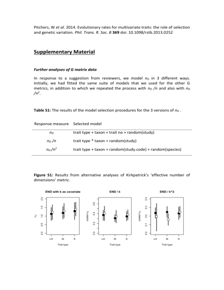
Pitchers, W et al. 2014. Evolutionary rates for multivariate traits: the role of selection
and genetic variation. Phil. Trans. R. Soc. B 369 doi: 10.1098/rstb.2013.0252
Supplementary Material
Further analyses of G matrix data
In response to a suggestion from reviewers, we model nD in 3 different ways.
Initially, we had fitted the same suite of models that we used for the other G
metrics, in addition to which we repeated the process with nD /n and also with nD
/n2.
Table S1: The results of the model selection procedures for the 3 versions of nD .
Response measure Selected model
nD
trait type + taxon + trait no + random(study)
nD /n
trait type * taxon + random(study)
nD /n2
trait type + taxon + random(study.code) + random(species)
Figure S1: Results from alternative analyses of Kirkpatrick’s ‘effective number of
dimensions’ metric.
Figure S2: Density of the number of traits for out 2 G matrix datasets. Note that in
both cases the majority of matrices are for between 4 & 6 traits. It is possible that
there are effects associated with the number of traits that we have been unable to
detect due to a lack of power. Only with a larger sample of larger matrices could we
test this.
Table S2: The counts of numbers of matrices of each size (in terms of number of
traits) represented in both our matrix datasets.
n
covariance matrix count
correlation matrix count
2
11
31
3
8
41
4
5
36
5
29
42
6
16
21
7
6
21
8
2
17
9
3
5
10
4
17
1
3
total
81
221
We mentioned in the Discussion section that one legitimate concern with a
quantitative review of the structure of G is that G can be challenging to estimate,
and extremely challenging to estimate well. In particular, a smaller-than-optimal
sample of families in a breeding design has the potential to inflate the magnitude of
the gmax, at the expense of the minor eigenvalues [55,56]. Given the importance of
the ‘lines of least evolutionary resistance’ and ‘genetic degrees of freedom’ concepts
for our thinking about multivariate evolution, it is a useful (not to mention
reassuring) finding that there is no evidence to suggest that these patterns are
driven by the sample sizes of the studies involved.
Figure S3: Pairs plot of the subset of covariance matrix measures that appear to
represent the structure (as opposed to the magnitude) of G, in addition to the
number of families measured to estimate G. (This plot does not include matrices
estimated using an animal model, only those that result from breeding designs.
‘families’ in this case was taken to mean the number of sires in a half-sib design and
the number of dams in parent-offspring regressions)
Figure S4: Pairs plot of the subset of correlation matrix measures that appear to
represent the structure (as opposed to the magnitude) of G, in addition to the
number of families measured to estimate G. (This plot does not include matrices
estimated using an animal model, only those that result from breeding designs.
‘families’ in this case was taken to mean the number of sires in a half-sib design and
the number of dams in parent-offspring regressions)
Further analyses of selection data
In the main MS we only reported our findings from linear selection gradient () data.
However, in the process of collecting these estimates we also tabulated estimates of
quadratic selection gradients (the diagonal elements of the  matrix). These
estimates were reported less frequently than those for , and there is a smaller
dataset to work with. We divided the quadratic gradients into to groups; negative
(potentially stabilizing) and positive (potentially disruptive) gradients. For each of
these subsets, we fit the same model as used for the  dataset (a formal Bayesian
meta-analysis following [38]: see main text), the results of which are visualized in
Figure S5 below. Firstly, we should note that there are no differences among trait
types or between taxa in which can have a high level of confidence. It is interesting
to not that, for both taxa, there appear to be different trends in the two subsets of
quadratic gradients, but we can say little more than that with the currently available
data.
Figure S5: Posterior means and 95% credible intervals for negative (left panel) and
positive (right panel) quadratic selection gradients. Trait types are life-history (LH),
morphology (M) and sexually selected (S) and filled points are for animals and open
points for plants.