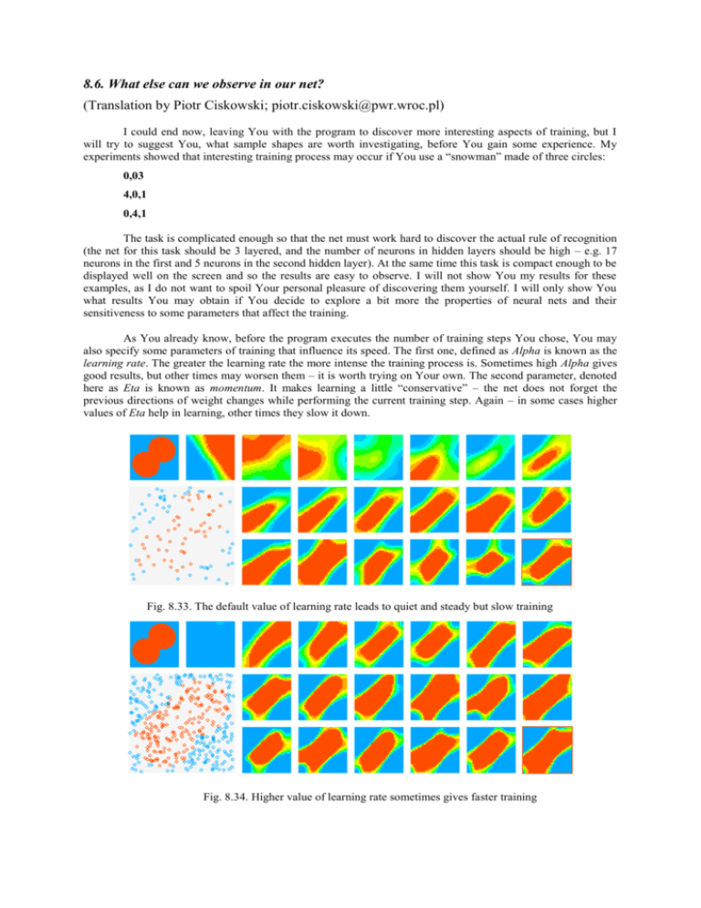
8.6. What else can we observe in our net?
(Translation by Piotr Ciskowski; piotr.ciskowski@pwr.wroc.pl)
I could end now, leaving You with the program to discover more interesting aspects of training, but I
will try to suggest You, what sample shapes are worth investigating, before You gain some experience. My
experiments showed that interesting training process may occur if You use a “snowman” made of three circles:
0,03
4,0,1
0,4,1
The task is complicated enough so that the net must work hard to discover the actual rule of recognition
(the net for this task should be 3 layered, and the number of neurons in hidden layers should be high – e.g. 17
neurons in the first and 5 neurons in the second hidden layer). At the same time this task is compact enough to be
displayed well on the screen and so the results are easy to observe. I will not show You my results for these
examples, as I do not want to spoil Your personal pleasure of discovering them yourself. I will only show You
what results You may obtain if You decide to explore a bit more the properties of neural nets and their
sensitiveness to some parameters that affect the training.
As You already know, before the program executes the number of training steps You chose, You may
also specify some parameters of training that influence its speed. The first one, defined as Alpha is known as the
learning rate. The greater the learning rate the more intense the training process is. Sometimes high Alpha gives
good results, but other times may worsen them – it is worth trying on Your own. The second parameter, denoted
here as Eta is known as momentum. It makes learning a little “conservative” – the net does not forget the
previous directions of weight changes while performing the current training step. Again – in some cases higher
values of Eta help in learning, other times they slow it down.
Fig. 8.33. The default value of learning rate leads to quiet and steady but slow training
Fig. 8.34. Higher value of learning rate sometimes gives faster training
Fig. 8.35. Too high learning rate ends up in oscillations
– the net in turns comes close to the desired solution, then goes away
Both mentioned coefficients are constantly accessible in the program window of Example 09, so You
may change them during training to observe interesting results. You may start with modifying them only once
before learning starts. You should notice how training speeds up with higher values of Alpha. E.g. fig. 8.33
presents the training process for some task with standard values, while fig. 8.34 shows training with higher
Alpha.
Too high Alpha is not good, however. Signs of instability occur, as it is perfectly illustrated in fig. 8.35. The way
to suppress the oscillations, which are always the result of a too high learning rate, is turning up the Eta
coefficient, that is momentum. If You wish, You may analyze the influence of changing momentum on training
and notice its stabilizing power when training goes out of control.
Fig. 8.36. The regions learned by the net do not match the desired ones
if we use a two-layer net
Fig. 8.37. Good solution found quickly by a three-layer net
Fig. 8.38. Signs of instability during learning of a three layer net
Another possible area of interesting research is the dependence of net’s behavior on its structure. To
analyze that You must choose a really tough problem to be learned. A good one is presented in fig. 8.4 and 8.5.
The difficulty here is the necessity of fitting into narrow and tight bays defined by the blue area of negative
answers. In order to fit to each of these slots a very precise choice of parameters is needed and that is really a big
challenge for the net.
A three layered net is able to distinguish all the subtle parts of the problem (fig. 8.37), although it is sometimes
difficult to keep the training stable, as it happens that the net – even being very close to the solution – moves
away of it due to the backpropagation of errors and searches for solution in another, incorrect, area where it
cannot find it (fig. 8.38)
Now You may use your imagination and freely define the regions where the net should react positively and
negatively. You may run tens of experiments and obtain hundreds of observations. Although I am warning You –
think of your precious time, as training a large net may take long time especially in its initial stages. What You
need is either a very fast computer or some patience. I am not forcing You what to choose, but just suggest that
the patience is cheaper…