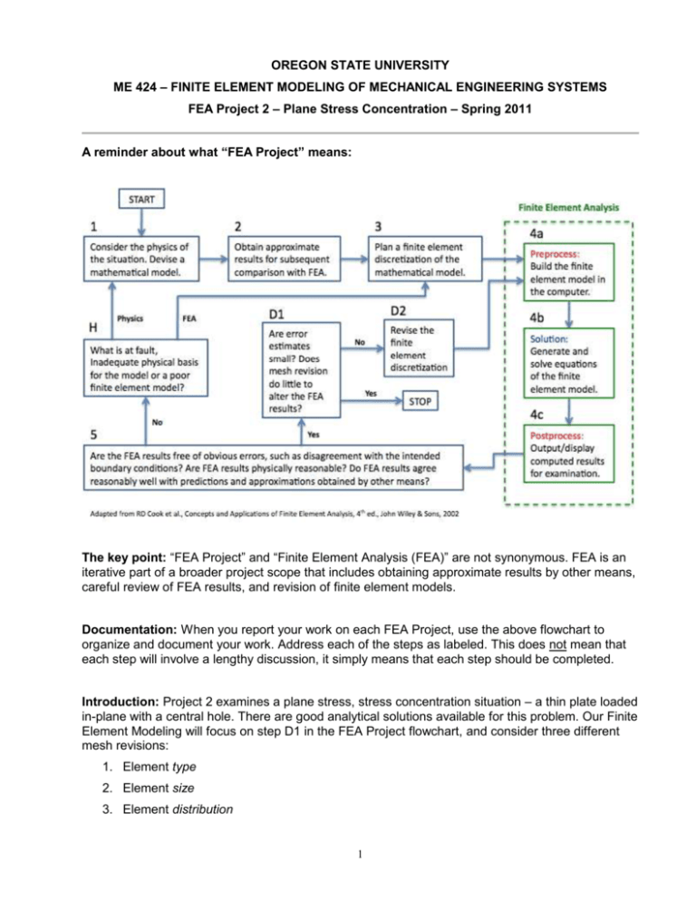
OREGON STATE UNIVERSITY
ME 424 – FINITE ELEMENT MODELING OF MECHANICAL ENGINEERING SYSTEMS
FEA Project 2 – Plane Stress Concentration – Spring 2011
A reminder about what “FEA Project” means:
The key point: “FEA Project” and “Finite Element Analysis (FEA)” are not synonymous. FEA is an
iterative part of a broader project scope that includes obtaining approximate results by other means,
careful review of FEA results, and revision of finite element models.
Documentation: When you report your work on each FEA Project, use the above flowchart to
organize and document your work. Address each of the steps as labeled. This does not mean that
each step will involve a lengthy discussion, it simply means that each step should be completed.
Introduction: Project 2 examines a plane stress, stress concentration situation – a thin plate loaded
in-plane with a central hole. There are good analytical solutions available for this problem. Our Finite
Element Modeling will focus on step D1 in the FEA Project flowchart, and consider three different
mesh revisions:
1. Element type
2. Element size
3. Element distribution
1
Problem Statement:
Here are some figures illustrating the geometry and stress concentration results:
2L
2h
From AC Ugural and SK Fenster, Advanced Strength and Applied Elasticity, 3rd ed., Prentice Hall, New Jersey, 1995.
Analytical Solution:
The elasticity solution, in polar coordinates:

1  a 2   3a 4 4a 2 
 r   01 2  1 4  2 cos2
2  r   r
r 

1
2

   01
 r


a 2   3a 4 

1
c
os2





r 2   r 4 


1  3a 4 2a 2 
   0 1 4  2 sin 2
2  r
r 
Coordinate transformation, from polar to Cartesian:
 x   r cos2    sin 2   2 r sin  cos
 y   r sin 2    cos2   2 r sin  cos
 xy   r   sin  cos   r cos2   sin 2  

Consult a Mechanics of Materials reference for Principal Value and Max Shear equations.
2
Matlab:
You will need to generate plots of stress from the analytical solution for comparison with your finite
element analysis. I recommend Matlab for this task. There is a small complication involved: Matlab
needs 2D information organized as matrices for generating plots with the standard tools.
Here is an outline of the Matlab process for calculating the results and creating display plots:
# create scalar variables that define the problem geometry
a = 1.0;
h = 5.0;
# create matrices of point locations in polar coordinates
[th,r] = meshgrid((90:5:180)*pi/180 , a:.1:h);
# convert the matrices of point locations to Cartesian coordinates
[X,Y] = pol2cart(th,r);
# calculate polar coordinate stresses from the analytical solution
sig_nom = 40.0;
sig_r = …;
sig_th = …;
tau_rth = …;
# convert to Cartesian coordinates
sig_x = …;
sig_y = …;
tau_xy = …;
# plot as filled contours against the Cartesian grid
figure(1); contourf(X,Y,sig_x,20);
figure(2); contourf(X,Y,sig_y,20);
figure(3); contourf(X,Y,tau_xy,20);
# find principals and max shear
sig_1 = …;
sig_2 = …;
tau_max = …;
# plot as filled contours
figure(4); contourf(X,Y,sig_1,20);
figure(5); contourf(X,Y,sig_2,20);
figure(6); contourf(X,Y,tau_max,20);
3
Finite Element Analysis:
Convergence for Generic Mesh: Create a single trimmed surface that represents the upper-left
quarter of the plate with a hole. The overall plate dimensions are:
2L = 30 mm
2h = 10 mm
2a = 2 mm
thickness = 1 mm
Model a steel plate with properties:
E = 200 GPA
 = 0.32
Enforce symmetry using displacement boundary conditions, and load with:
0 = 40 MPa
The goal for the convergence study is to fill-in the following table and create corresponding graphs
of maximum model displacement and maximum x-component stress vs. number of nodes in the
model.
Tri3
# nodes in model
Maximum model displacement (mm)
Maximum x-component stress (MPa)
Maximum model displacement (mm)
Maximum x-component stress (MPa)
Maximum model displacement (mm)
Maximum x-component stress (MPa)
~ 75 (report actual number)
~ 200 (report actual number)
~ 500 (report actual number)
~ 1000 (report actual number)
Tri6
# nodes in model
~ 75 (report actual number)
~ 200 (report actual number)
~ 500 (report actual number)
~ 1000 (report actual number)
Quad8
# nodes in model
~ 75 (report actual number)
~ 200 (report actual number)
~ 500 (report actual number)
~ 1000 (report actual number)
4
Meshing:
Use Mesher – Paver to create the nodes and elements. Be sure you have Element Shape and
Topology set correctly. Control the mesh density by un-checking Automatic Calculation and setting
Global Edge Length – Value manually. You do not have to hit the suggested number of nodes
(ranging from 75 to 1000) exactly, but do record the actual number created for each model. The
simplest way to accomplish this is to guess a value for global edge length, create the mesh, Undo if
the density is far from the target, and adjust the value accordingly.
Go to the Analysis tab and Delete – Results Attachment if a previous analysis exists. Then run the
model, attach the new results, and go to the Results tab. Create a Deformation plot, then use the
Cursor tool (set to Nodes) to establish the maximum displacement magnitude (it should be in the
upper-left corner). Next create a Fringe plot of the x-component stress, and again use the Cursor
tool (set to Nodes) to establish the maximum x-component stress magnitude (should be near the top
of the hole.) Note that the node with the maximum stress may be a mid-side node for a higher-order
element.
Be Creative:
The final analysis I would like you to conduct is your creation of an accurate and efficient mesh for
this problem. Use the results of your convergence study and the Mesh Seeds tool in Patran to
concentrate nodes in the region of the hole. Do not just create a ridiculously refined mesh that
covers the entire problem domain. Use element type and element density effectively to generate
detailed fringe plots of stress for the problem.
Hand In (Thursday, April 28):
1. A report that addresses each point in the project flowchart. This project emphasizes D1, so
the most content and detail will reside there, but address all steps.
2. Include your convergence table, and plots of Displacement vs. # Nodes and Stress vs.
Number of nodes. Fit appropriate trendlines to the data series in the plots.
3. Summarize calculation of the expected result, and create filled contour plots of stress tensor
components and principal/max shear invariants. Make sure these plots include range values.
4. Create corresponding fringe plots of stress for your model developed under “Be Creative.”
Also document the model with a figure that shows the mesh and all boundary conditions.
5. Also discuss the following:
a. Why did I ask for convergence plots vs. # nodes and not vs. # elements?
b. Do your convergence plots behave as you expected? How does the displacement
plot differ from the stress plot?
c. Which had more impact for this problem, refinement of # nodes or refinement of
element order? Explain.
d. Critically compare your plots of the analytical solution with the FEA solution (compare
and contrast; how do they agree, how do they differ.)
e. Draw and support a conclusion: did FEA do a good job with this problem?
5