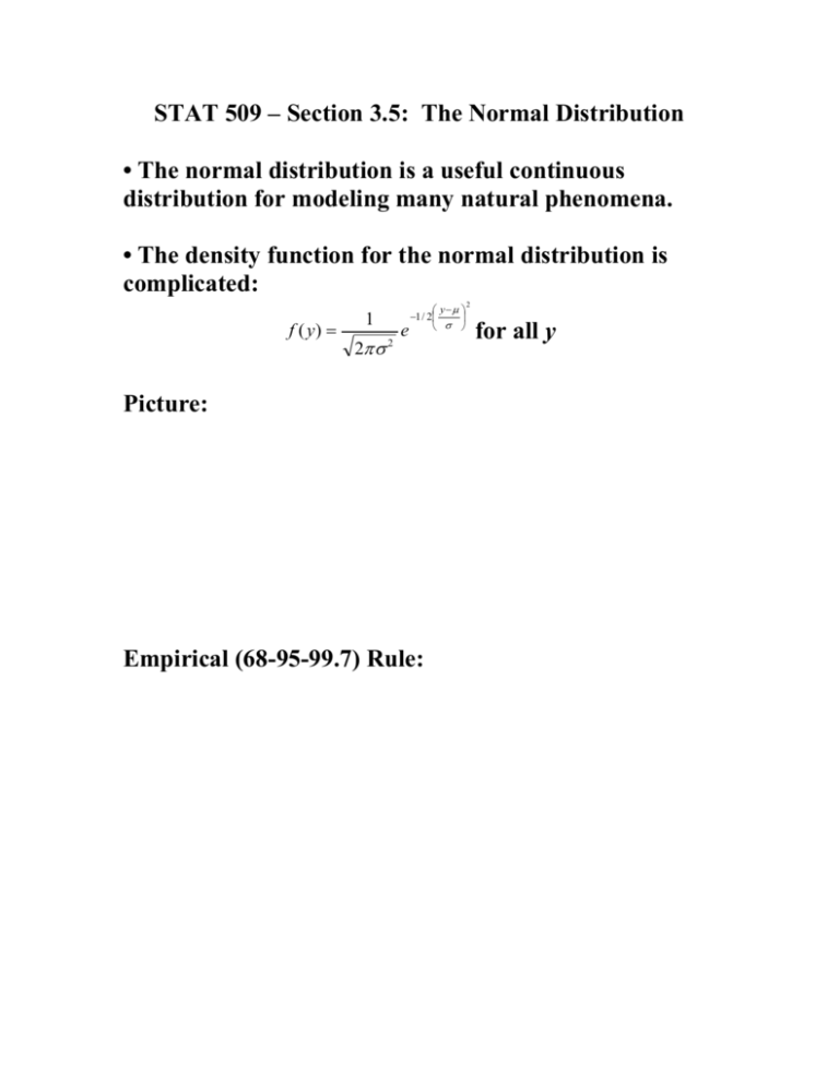
STAT 509 – Section 3.5: The Normal Distribution
• The normal distribution is a useful continuous
distribution for modeling many natural phenomena.
• The density function for the normal distribution is
complicated:
f ( y) 
1
2 2
e
 y 
1 / 2 

  
Picture:
Empirical (68-95-99.7) Rule:
2
for all y
Example: Since 1900, the magnitude of earthquakes
that measure 0.1 or higher on the Richter Scale in a
certain location in California is distributed
approximately normally, with μ = 6.2 and σ = 0.5,
according to data obtained from the United States
Geological Survey.
Picture:
What percentage of such earthquakes are above 5.7 on
the Richter Scale?
What percentage of such earthquakes are between 5.2
and 7.2 on the Richter Scale?
What percentage of such earthquakes are between 5.7
and 7.7 on the Richter Scale?
What percentage of such earthquakes are between 6.7
and 7.7 on the Richter Scale?
Note that the density changes depending on the values
of the mean  and the variance , so there are many
different normal distributions (change  and/or , get a
different distribution).
• Changing  shifts the distribution to the left or right.
• Increasing  makes the normal distribution wider.
• Decreasing  makes the normal distribution
narrower.
Standard Normal Distribution [Notation: N(0, 1)]: The
normal distribution with mean  = 0 and standard
deviation  = 1 (hence variance  = 1 also).
Picture:
Note: N(0, 1) distribution sometimes called the
“z-distribution” and standard normal values are
denoted by z.
Table 1 in back of book gives area to the left of certain
listed values of z.
Example: Area under N(0, 1) density to left of 1.24:
Table IV: Go to row labeled 1.2, column labeled .04:
Correct area =
What does this area mean?
• If Z is a r.v. with a standard normal distribution, then
P(Z < 1.24) =
[Note: Same as P(Z ≤ 1.24).]
• We expect that 89.25% of the values of data having a
standard normal distribution will be less than 1.24
Other Probabilities:
P(Z > 1.24) =
P(0 < Z < 1.24) =
Other examples:
P(-0.54 ≤ Z < 0) =
P(-1.75 < Z < -0.79) =
P(-0.79 < Z < 1.16) =
Finding standard normal probabilities in R:
> pnorm(1.24)
[1] 0.8925123
Finding Probabilities for any Normal r.v.
Standardizing: If a r.v. Y has a normal distribution
with mean  and standard deviation , then the
standardized variable
Z=Y–

has a standard normal distribution.
So: We can convert any normal r.v. to a standard
normal and then use Table 1 to find probabilities!
Example: The thickness of a certain steel bolt that
continuously feeds a manufacturing process is normally
distributed with a mean of 10.0 mm and standard
deviation of 0.3 mm. Manufacturing becomes
concerned about the process if the bolts are thicker than
10.5 mm or thinner than 9.5 mm.
If the process is following the assumed distribution,
what is the probability that a randomly selected bolt is
either thicker than 10.5 mm or thinner than 9.5 mm?
What is the probability that a randomly selected bolt is
thicker than 10.8 mm?
We can also find the particular value of a normal r.v.
that corresponds to a given proportion.
Example: Assuming the process is going correctly,
approximately 1% of the bolts produced will have
thicknesses less than ______.
We need to “unstandardize” to get back to the Y value
(bolt thickness).
General Rule: To unstandardize a z-value, use:
Y = Z + 
More Normal Probabilities
Example: Recall the earthquake magnitudes were
distributed approximately normally, with μ = 6.2 and σ
= 0.5.
• What proportion of earthquakes are greater than 7?
• What is the probability that a randomly selected
earthquake is between 5.0 and 6.0 on the scale?
• The middle 75% of earthquake measurements are
between what two values on the Richter scale?
• The normal model is not appropriate for every data
set.
• It tends to give a decent approximation to the behavior
of many variables observed in nature.
• Why? Many natural phenomena are in fact the sum
total of lots of different factors that act independently to
produce the final value.
• We will see that the normal distribution can be
theoretically justified as a model for the sum of many
independent quantities.