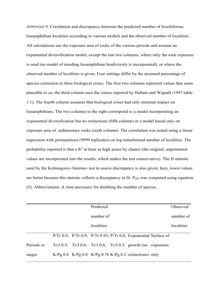
APPENDIX 9. Correlation and discrepancy between the predicted number of fossiliferous
lissamphibian localities according to various models and the observed number of localities.
All calculations use the exposure area of rocks of the various periods and assume an
exponential diversification model, except the last two columns, where only the rock exposure
is used (no model of standing lissamphibian biodiversity is incorporated), or where the
observed number of localities is given. Four settings differ by the assumed percentage of
species extinction in three biological crises. The first two columns represent values that seem
plausible to us; the third column uses the values reported by Hallam and Wignall (1997:table
1.1). The fourth column assumes that biological crises had only minimal impact on
lissamphibians. The two columns to the right correspond to a model incorporating an
exponential diversification but no extinctions (fifth column) or a model based only on
exposure area of sedimentary rocks (sixth column). The correlation was tested using a linear
regression with permutations (9999 replicates) on log-transformed number of localities. The
probability reported is that a R2 at least as high arises by chance (the original, unpermuted
values are incorporated into the results, which makes the test conservative). The D statistic
used by the Kolmogorov-Smirnov test to assess discrepancy is also given; here, lower values
are better because this statistic reflects a discrepancy in fit. P(D) was computed using equation
(5). Abbreviations: d, time necessary for doubling the number of species.
Predicted
Observed
number of
number of
localities
localities
P/Tr 0.9; P/Tr 0.9; P/Tr 0.95; P/Tr 0.8; Exponential Surface of
Periods or
Tr/J 0.5; Tr/J 0.6; Tr/J 0.8; Tr/J 0.5; growth (no exposures
stages
K/Pg 0.8 K/Pg 0.8 K/Pg 0.76 K/Pg 0.2 extinctions) only
(d 18.53 (d 18.21 (d 16.65
(d 25.20
Ma)
Ma)
Ma)
Ma)
Triassic
0.27
0.29
0.23
0.25
0.48
47.15
2
Jurassic
3.10
2.81
1.37
2.12
5.40
149.83
18
16.32
15.23
8.79
8.29
14.74
127.12
23
Cretaceous
54.43
51.91
33.71
22.81
33.08
94.44
35
Paleocene
14.75
14.29
12.06
21.17
30.58
63.62
15
Eocene
61.49
60.23
54.06
79.50
101.37
143.63
56
Oligocene
55.16
54.58
51.72
64.86
73.6
71.29
66
Miocene
154.97
154.86
154.78
166.29
168.97
116.07
210
Pliocene
45.12
45.38
46.94
45.59
43.00
23.12
96
718.79
724.15
756.13
714.49
660.77
333.67
466
82.59
83.26
87.21
81.65
75.00
37.07
220
Early
Cretaceous
Late
Pleistocene
Holocene
R2(log-transformed) 0.892
0.894
0.897
0.882 0.865
0.058
P(log-transformed) 0.0001
0.0001
0.0001
0.0001 0.0001
0.4746
D
0.1138
0.1133
0.1304
0.1146
0.1201
3.36 E5.17 E-14 7.00 E-14 3.06 E-18
P(D)
0.3994
1.18 E-
1.48 E-15
14
167
METHODOLOGICAL NOTE
The map uses a coarse geological scale (i.e. “Upper Paleozoic” or “Jurassic and
Cretaceous”). To maximize the power of our statistical tests for verifying that the assumptions
required by the method (Marshall, 1997) were met, we thought that it was preferable to
estimate the area covered by sediments for shorter periods. Thus, we assumed that the amount
of sediment covered by any period was proportional to its duration. For instance, the
Paleocene lasted 9.7 Ma and the “Tertiary” lasted 63.7 Ma, so we inferred that the area of
Paleocene sediments equaled 0.152 times the area covered by the “Tertiary” (0.152 = 9.7
Ma/63.7 Ma). The only exception is for the “Quaternary”; instead of giving the Holocene a
minute proportion of the “Quaternary” (0.0115 Ma/1.806 Ma = 0.0064), we arbitrarily
assigned it 0.1 of the “Quaternary” record, to compensate for the much greater sampling effort
that results from the archaeozoological research on historic, protohistoric and late prehistoric
sites. This procedure cannot have reduced the power of the test because the KolmogorovSmirnov goodness-of-fit test uses the maximal observed difference between predicted and
observed values (here, the cumulated number of fossiliferous localities at various periods,
starting in the Triassic), and our method does not affect this difference for any of the times for
which it can be unambiguously established using the geological map (at the end of the
Triassic, at the end of the Cretaceous, and at the end of the Pliocene). The only partial
exception is for the end of the Pliocene because part of the Cenozoic sediments are identified
only as undifferentiated Cenozoic, so we had to assume that part of this was from the
Pleistocene and Holocene. Thus, our interpolation of the area covered by sediments for
shorter periods can only increase the power of the Kolmogorov-Smirnov test; it cannot have
adverse effects on any other calculations. This procedure also enables us to assess better the
quality of the fit of our recovery potential function using linear regressions.
The proportions of lissamphibians becoming extinct in the three great biological crises are
based on statistics that reflect mostly marine metazoans. It might be objected that the
extinction levels of lissamphibians many not have been comparable to those of marine
metazoans, which have been most intensively studied (Hallam and Wignall, 1997), but this
matters little because we only need to get a good match between the expected and observed
number of localities, and we have tested the quality of this fit (see below). The proportion of
species-level extinction reported for metazoans yields plausible potential recovery curves and
is incorporated into our models.
The resulting potential recovery values can also be divided by the duration of a given
geological period as a proxy of average standing lissamphibian biodiversity. This approach
seems more appropriate than directly using the fossil recovery potential calculated for a
period based on the exponential diversification model because the latter would result in a high
potential if a period were very long. In fact, the length of the period is irrelevant; what matters
is the abundance of lissamphibians in the former biological communities, and the area of
exposed fossiliferous rocks. Whether these rocks represent e.g. 1 Ma or 10 Ma should have no
impact on the recovery potential.
The estimated average biodiversity in each period can be multiplied by the area of
exposures of rocks of various periods on the continents to yield the potential recovery curve;
this is the method that was adopted here. With this model, we should be able to determine if
the fossil record of lissamphibians is consistent with our starting assumption of lissamphibian
origin (i.e. the timing suggested by Zhang et al., 2005) and diversification. We have found
that our recovery potential function is adequate using a Kolmogorov-Smirnov test of
goodness of fit for continuous distributions. The exact probability for the values of D at such
our high sample size (n = 1207) is not reported in Zar (1984), but it can be computed by
isolating α (the probability threshold) in the formula used when n is large:
Dα n = ([-ln(α/2)]2n)-1/2
(4)
This equation becomes:
2
α = 2ε-2nD
In this case, what is computed is a probability (α = p).
(5)
We have also tested the correlation between the observed number of localities and the
predicted number of localities using our recovery potential functions using a simple linear
regression in Statview (Caldarola et al., 1998) and using a regression with permutations in
Permute (Casgrain, 2005). We tested normality using Progiciel R (Casgrain et al., 2004).
Since the distribution of the localities in the various periods was log-normal rather than
normal, the values were log-transformed.
Extinctions in the recovery potential curve.—Incorporation of extinction events into the
models is supported to an extent by the literature and by our new analyses. Among taxa that
have been interpreted as stem-amphibians, temnospondyls suffered a great reduction in
biodiversity towards the end of the Permian, although their record is not good enough to
determine if this was a slow decline or a result of the end-Permian crisis (Milner, 1990, 1991).
The “lepospondyls” also declined steadily in diversity in the Permian, but in their case, the
extinctions seem to have occurred well before the end of the Permian (contra Zhang et al.,
2005:fig. 2, 3) because only a few species persist into the Middle to Late Permian (Carroll,
2000). Less is known about how lissamphibians fared in times of biological crises. Aquatic
vertebrates, especially those living in fresh water, may have been little affected by the K/Pg
boundary event (Clemens, 1982; Fara, 2000); however, this conclusion is based mostly on
turtles and crocodilians, which have a much better fossil record.
REFERENCES
Caldarola, J., J. Gagnon, K. Haycock, J. Roth, C. Soper, and E. Wasserman. 1998. Statview,
version 5.0. SAS Institute.
Carroll, R. L. 2000. Lepospondyls. Pages 1198–1269 in Amphibian Biology (H. Heatwole,
and R. L. Carroll, eds.). Surrey Beatty & Sons, Chipping Norton.
Casgrain, P. 2005. Permute!, version 3.4 alpha. Available at
http://www.bio.umontreal.ca/Casgrain/en/labo/permute/index.html
Casgrain, P., P. Legendre, and A. Vaudor. 2004. The R Package for multidimensional and
spatial analysis. Available at
http://www.fas.umontreal.ca/BIOL/Casgrain/en/labo/R/v4/progress.html
Clemens, W. A. 1982. Patterns of extinction and survival of the terrestrial biota during the
Cretaceous/Tertiary transition. Pages 407–413 in Geological Implications of Impacts
of Large Asteroids and Comets on the Earth (L. T. Silver, and P. H. Schultz, eds.). The
Geological Society of America, Boulder.
Fara, E., and M. J. Benton. 2000. The fossil record of Cretaceous tetrapods. Palaios 15:161–
165.
Hallam, A., and P. Wignall. 1997. Mass Extinctions and their aftermath. Oxford University
Press, Oxford.
Marshall, C. R. 1997. Confidence intervals on stratigraphic ranges with nonrandom
distributions of fossil horizons. Paleobiology 23:165–173.
Milner, A. R. 1990. The radiations of temnospondyl amphibians. Pages 321–349 in Major
Evolutionary Radiations (P. D. Taylor, and G. P. Larwood, eds.). Clarendon Press,
Oxford.
Milner, A. R. 1991. Lydekkerinid temnospondyls—relationships and "extinction" in Fifth
Symposium on Mesozoic Terrestrial Ecosystems and Biota, Oslo. 364:49–50.
Zar, J. H. 1984. Biostatistical Analysis, 2nd edition. Prentice-Hall, Englewood Cliffs, New
Jersey.
Zhang, P., H. Zhou, Y.-Q. Chen, Y.-F. Liu, and L.-H. Qu. 2005. Mitogenomic perspectives on
the origin and phylogeny of living amphibians. Syst. Biol. 54:391–400.