Ocean Data View – Presentations and Exercises
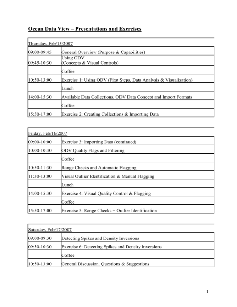
Thursday, Feb/15/2007
09:00-09:45
09:45-10:30
General Overview (Purpose & Capabilities)
Using ODV
(Concepts & Visual Controls)
Coffee
10:50-13:00
Exercise 1: Using ODV (First Steps, Data Analysis & Visualization)
Lunch
14:00-15:30
Available Data Collections, ODV Data Concept and Import Formats
Coffee
15:50-17:00
Exercise 2: Creating Collections & Importing Data
Friday, Feb/16/2007
09:00-10:00
Exercise 3: Importing Data (continued)
10:00-10:30
ODV Quality Flags and Filtering
Coffee
10:50-11:30
Range Checks and Automatic Flagging
11:30-13:00
Visual Outlier Identification & Manual Flagging
Lunch
14:00-15:30
Exercise 4: Visual Quality Control & Flagging
Coffee
15:50-17:00
Exercise 5: Range Checks + Outlier Identification
Saturday, Feb/17/2007
09:00-09:30
Detecting Spikes and Density Inversions
09:30-10:30
Exercise 6: Detecting Spikes and Density Inversions
Coffee
10:50-13:00
General Discussion. Questions & Suggestions
1
Exercise 1:
1. Copy the directories under \SeaDataNet\Reiner Schlitzer to a work directory
on your local hard disk.
2. Install the optional package odvmpOP_coastRegional_w32.zip from
http://odv.awi.de. This package contains high resolution regional coastlines for the
Mediterranean, Baltic, North Sea and other regions.
3. Run ODV and open the MedatlasII_Btl collection on your hard disk. Make the map to
use the MeditHR coastlines installed during step 2. Invoke ODV Help and read the
chapter on map Display Options for instructions on how to do this.
4. In MAP mode produce full screen maps of (a) all stations in MedatlasII_Btl, (b) of all
stations containing data for Phosphate, and (c) of all stations containing data for
Phosphate and Nitrate. Save the configuration of (a). Use a descriptive name for the
configuration, such as AllStationsMap. How many stations have Phosphate and
Nitrate data?
5. Load the AllStationsMap configuration saved during (4) and make Display Option
changes, e.g., size and color of station dots, map projection, coastline/bathymetry layers
etc. Save your favourite configuration. Undo last configuration changes.
6. Switch to STATION mode and produce plots with temperature, salinity and oxygen
profiles. Change the window layout so that you only have two large windows. Change the
variables on x and y axis. What are typical oxygen values in 200 m depth in the Black Sea
and Meditterranean?
7. (Advanced) Specify a station selection rectangle or polygon to select only stations in a
region of interest. Define Potential Temperature as a derived variable. Switch to
SCATTER mode and produce a large T/S diagram with salinity on x and Tpot on y.
Define Potential Density as second derived variable and define a second window showing
profiles of potential density. Do you see any suspicious data?
8. (Advanced) Switch to STATION mode and undo any regional station selection from step
7. Switch to SECTION mode and define your favourite section. Produce section plots of
potential temperature, salinity and oxygen. Also create a T/S diagram of the section data.
Add contour lines to the section plots and produce GIF, PNG or JPG image output.
Exercise 2:
1. Create a new directory profileCollection on your local hard disk and create a
new ODV collection in this directory using ODV’s File>New option. Choose
a name for the new collection, e.g., MyProfiles. When prompted for the
definition of variables in the collection choose Medatlas Bottle
variables. Note that the newly created collection is empty, initially.
2. Import some Medatlas bottle data from file b0653311.987 in the
\SeaDataNet\Reiner Schlitzer\importData directory. Use option
Import>Medatlas Format Files>Profile Data>Single File. Then use option Full Domain
from the map’s popup menu to adjust the domain covered by the imported stations. Undo
last change before proceeding.
3. (Advanced) Import data from the US NODC World Ocean Database 2005 file
OSDO1985.gz. Use option Import>NODC Formats>World Ocean Database>Single
File. On the Import Options dialog note that the WOD 2005 import file provides values
2
for Depth [m] while the collection stores Pressure [decibars]. Therefore, depths have to
be converted to pressure values during import. Use the ODV help to find out how to do
this. Don’t forget to associate or convert other variables as well. Also note that units for
the nutrients in the source file and target collection appear to be different. Do we need to
convert these?
4. (Advanced) Download ARGO float profile data from
http://www.coriolis.eu.org/cdc/argo.htm and import them using Import>ARGO
Formats>Float Profiles (…)>Single File.
5. Create a new directory time-seriesCollection on your local hard disk and
create a new ODV collection in this directory using ODV’s File>New option.
Choose a name for the new collection, e.g., MyTimeSeries. When prompted
for the definition of variables in the collection choose Medatlas Time
Series variables. Note that the newly created collection is empty,
initially.
6. Import some Medatlas current meter data from file
example_medatlas_time_series.dat in the \SeaDataNet\Reiner
Schlitzer\importData directory. Use option Import>Medatlas Format
Files>Time Series Data>Single File. Then use option Full Domain from the map’s popup
menu to adjust the domain covered by the imported stations. Undo last change before
proceeding.
7. Produce plot of current speed versus time.
Exercise 3:
1. If not already present create an ODV desktop icon.
2. Drag the file data_from_WoceBtl.txt from \SeaDataNet\Reiner
Schlitzer\importData\speadsheet onto the ODV icon. Note that ODV created
a new collection data_from_WoceBtl and imported the data from the .txt file in a single,
automatic step. This was possible because data_from_WoceBtl.txt adheres to the
ODV Generic Spreadsheet format. Any such file can be simply dragged onto the ODV
icon and can be imported automatically.
3. Drag your own data file onto the ODV icon. Is it imported automatically? Does it adhere
to the ODV Generic Spreadsheet format? (See help file for format specification.) Ask for
help if you are stuck.
3
Exercise 4:
1. Drag the file data_from_WoceBtl_compact_noQF.txt from
\SeaDataNet\Reiner Schlitzer\qualityCheck onto the ODV icon. Produce
section plots of Nitrate and Silicate with the unchecked data (Display Options settings:
Gridded Field, VG Gridding, 30 and 25 for X and Y scale lengths). Save these sections to
image files for comparison with the cleaned sections later.
2. Switch to SCATTER mode and visually quality control the data. Note that you can use
different kinds of plots to identify outliers, e.g., profiles, T/S plots or general
property/property plots, such as for instance Phosphate versus Oxygen or Phosphate
versus Nitrate. Some cases are difficult to decide and you may want to look at several
plots simultaneously. Start with quality control of Nitrate and Silicate, then do the other
variables if time permits.
3. Exclude Questionable and Bad data by applying data quality filters and redo the Nitrate
and Silicate sections. Any improvement?
4. Apply visual data quality control to your own dataset.
Exercise 5:
1. Drag the file xbt_noQF.txt from \SeaDataNet\Reiner
Schlitzer\qualityCheck onto the ODV icon. Switch to SCATTER mode and
make sure you have a large plot window with temperature profiles.
2. Note that some XBT locations fall on land. Lets assume you know the correct
longitude/latitude values. Edit the metadata of these XBTs accordingly using the Edit
Header option of the text window popup menu.
3. Start cleaning the XBT data by applying range checks.
4. By clicking into the data plot try to find profiles that look good over some depth range but
have questionable or bad data above or below (if you can’t find one select station # 1248).
Do questionable or bad quality flagging for the entire set of problematic values. Note that
it may be useful to select a regional subset of stations before doing the quality control.
Exercise 6:
1. Open the xbt_noQF collection from exercise 5 again.
2. Define the Vertical Derivative of Temperature as a derived variable and create a window
layout with one large plot for temperature profiles and another window with d/dz
Temperature versus depth.
3. In the latter window click on points with very large positive or negative d/dz Temperature
values to identify spikes. Manually edit the quality flags of the bad data.
4