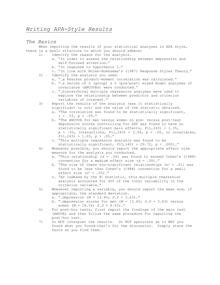
Writing APA-Style Results
The Basics
When reporting the results of your statistical analyses in APA style,
there is a basic structure to which you should adhere:
1)
Identify the reason for the analysis.
a. “In order to assess the relationship between depression and
self-focused attention…”
b. “In response to hypothesis 1…”
c. “In line with Nolen-Hoeksema’s (1987) Response Styles Theory…”
2)
Identify the analysis you used.
a. “…a Pearson product-moment correlation was calculated.”
b. “…a series of 2 (group) x 2 (pre/post) mixed model analyses of
covariance (ANCOVAs) were conducted.”
c. “…hierarchical multiple regression analyses were used to
explore the relationship between predictor and criterion
variables of interest.”
3)
Report the results of the analysis (was it statistically
significant or not) and the value of the statistic obtained.
a. “The correlation was found to be statistically significant,
r = .53, p < .05…”
b. “The ANCOVA for men versus women on pre- versus post-test
depression scores controlling for SES was found to have no
statistically significant main effects, F(1,243) = 1.35,
p > .05, interactions, F(1,243) = 2.06, p > .05, or covariates,
F(1,243) = 1.03, p > .05…”
c. “This multiple regression analysis was found to be
statistically significant, F(3,140) = 29.72, p < .0001…”
4)
Whenever possible, you should report the appropriate effect size
measure for the analysis you conducted.
a. “This relationship (d = .56) was found to exceed Cohen’s (1988)
convention for a medium effect size (d = .50).”
b. “The size of these non-significant relationships (η2 = .01) was
found to be less than Cohen’s (1988) convention for a small
effect size (η2 = .05).”
c. “As indexed by the R2 statistic, this multiple regression
analysis accounted for 40% of the total variability in the
criterion variable…”
5)
Whenever reporting a variable, you should report the mean and, if
appropriate, the standard deviation.
a. “…depression (M = 13.45; S.D = 3.43)…”
b. “…depression scores for men (M = 13.45; S.D = 3.43) versus
women (M = 18.54; S.D = 6.43)…”
6)
For post-hoc tests, first report the findings of the main test
(ANOVA) and then follow the same procedure for reporting the
post-hoc test.
7)
Do NOT interpret the results. Do NOT speculate as to WHY you
found what you found—that’s for the discussion. Simply state the
facts as you find them.
Examples
Below you will find several examples of APA style results. These are
results I myself wrote many years ago when I was in your position—namely,
undergraduate statistics. If you can meet this weak standard, you will be
well on your way to competently reporting the findings of your analyses.
Please note however; these are only examples and are not always “perfect.”
There is no such thing as perfect—you should try to balance a clear
communication of the results with the points outlined above.
Repeated Measures t-Test
In order to compare pre- versus post-test social dominance orientation
scores a repeated measures t-test was conducted. This test was found to be
statistically significant, t(57)=-2.67, p < .01, suggesting that there is a
strong relationship between an individual’s score on the first test (M =
33.69) as compared to the score on a later test (M = 37.60). The strength of
the relationship between the two test scores was .50 as indexed by η2.
One-Way Analysis of Variance (One-Way ANOVA)
A one-way analysis of variance compared the measure of social distance,
an emergent characteristic of social dominance orientation, to 3 groups of
people ranked by degree as to how much they agreed with being classified as
“inducers”; 1 category for people who agreed, one category for those who
disagreed, and a final category for those who neither agreed nor disagreed.
This analysis was found to be statistically non-significant, F(2, 55) = 2.09,
p < .13. The strength of the relationship, as indexed by η2, was .07. A
Tukey HSD further indicated that there was no significant relationship
between the variables.
Two-Way Analysis of Variance (Two-Way ANOVA)
Social distance scores were subjected to a 2 (high versus low social
dominance) x 2 (high versus low inducer class) two-way analysis of variance
in order to test the relationship between social dominance and inducer class.
All effects were found to be statistically non-significant. The main effect
of high social dominance scores was such that high inducer-identification
individuals were not significantly affected in social distance (M = 7.1)
while the low inducer-identification individuals demonstrated showed the same
lack of effect (M = 8.82), F(1,54) = .003, p < .90. The strength of this
relationship, as indexed by η2, was .02.
The main effect of high class identification was such that high social
dominance individuals were neither effected in social distance (M = 8.3)
while low social dominance individuals showed the same lack of effect (M =
8.14), F(1,54) = 3.24, p < .074. The strength of this relationship, as
indexed by η2, was.06. Owing to the lack of significant main effects or
interactions, no further post-hoc tests were performed.
Pearson Product-Moment Correlations
A Pearson product-moment correlation explored the relationship between
self-esteem (M = 19.2) and sports-related self-esteem (M = 17.2). This
analysis was found to be statistically significant, r(127) = .52, p < .01,
indicating a strong positive relationship between general self-esteem and
sports-related self-esteem. The strength of this relationship, as indexed by
eta2, was found to be .27.
Partial Correlation
This relationship [the correlation above] was then subjected to a
first-order partial correlation in order to explore the relationship
controlling for the effects of social support. The first-order correlation
was found to be statistically significant, r(53) = .35, p < .01, indicating
that a relationship between self-esteem and sports self-esteem exists above
and beyond the effects of social support, but that the relationship is
lessened; that is, social support affects both self-esteem and sports selfesteem and is closely related to the two.
Multiple Regression
A multiple regression was performed utilizing sports self-esteem as the
criterion and self-esteem and masculinity as predictors in order to determine
if sports self-esteem scores could be predicted as a function of general
self-esteem scores and masculinity. The analysis was found to be
statistically significant F(118) = 73.24, p < .01, indicating that selfesteem and masculinity are good predictors of sports-related self-esteem.
This multiple regression accounted for 55% of the variability, as indexed by
the adjusted R2 statistic. The regression equation for predicting sports
self-esteem from self esteem as an index of masculinity was found to be Y
= .48x1 + .28x2 - 1.89. The variable of masculinity, as indexed by its β
value of .59, was shown to have the strongest relationship to sports selfesteem.
Chi-Square Contingency Table Test
A 2 (gender) x 3 (experimental condition) χ2 test was conducted to test
the equal distribution of men versus women across experimental conditions.
This analysis was and found to be statistically non-significant, χ2 (2,54)
= .23, p < .89. The observed frequencies for the six cells can be found in
Table 1 [I did not include Table 1—it’s just a 2x3 table]. As indexed by
Cramér’s statistic, the strength of the relationship was .06.
MANOVA Analyses
It was hypothesized that measures of disordered eating, as indexed by
the Eating Attitudes Test (EAT), weight management behavior, and scores on
the Stunkard body image test would not be systematically related to an
individual’s involvement with fashion magazines and the attitudes and
behaviors such magazines support. Two groups, designated as “high” and “low”
magazine involvement were created by summing 7 questions, measured on a 3
point scale (1 = read it regularly; 2 = glance through it sometimes; 3 =
never read it), of interest in popular fashion magazines (i.e. Sassy, Glamour,
and Vogue). Participants were assigned to each group according to the mean
score of the sample (M = 11.91); individuals above the mean were designated
as having “high” magazine involvement, individuals below the mean were placed
in the “low” magazine involvement group. In that the variables of disordered
eating, weight management behavior, and body image are likely to be highly
correlated--and that the effect for the sum of variables was desired--a
multivariate analysis of variance (MANOVA) was conducted on these variables
across the groups of high and low magazine involvement.
Results from this MANOVA demonstrated a significant multivariate effect
for the relationship, Hotelling’s T(3, 262) = 6.79, p < .001. Univariate
results for this relationship demonstrated a significant effect for EAT score,
F(1, 264) = 7.33, p < .007, and weight loss method, F(1, 264) = 18.15, p
< .001; results for body image were non-significant, F(1,264) = .24, p < .63.
[you would want to report the effect sizes here but I, in my youth, neglected
to do so]