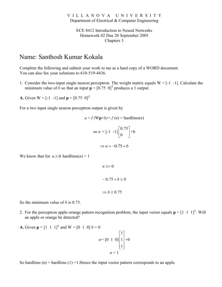
V I L L A N O V A U N I V E R S I T Y
Department of Electrical & Computer Engineering
ECE 8412 Introduction to Neural Networks
Homework 02 Due 20 September 2005
Chapters 3
Name: Santhosh Kumar Kokala
Complete the following and submit your work to me as a hard copy of a WORD document.
You can also fax your solutions to 610-519-4436.
1. Consider the two-input single neuron perceptron. The weight matrix equals W = [-1 -1]. Calculate the
minimum value of b so that an input p = [0.75 0]T produces a 1 output.
A. Given W = [-1 -1] and p = [0.75 0]T
For a two input single neuron perceptron output is given by
a = f (Wp+b)= f (n) = hardlims(n)
0.75
so n = [-1 -1] 
 +b
0 
 n  0.75  b
We know that for n  0 hardlims(n) = 1
n  0
 0.75  b  0
 b  0.75
So the minimum value of b is 0.75.
2. For the perceptron apple-orange pattern recognition problem, the input vector equals p = [1 1 1]T. Will
an apple or orange be detected?
A. Given p = [1 1 1]T and W = [0 1 0] b = 0
1
n= [0 1 0] 1 +0

1
n=1
So hardlims (n) = hardlims (1) =1.Hence the input vector pattern corresponds to an apple.
3. Calculate Euclidean distance from p = [1 1 1]T to each prototype vector.
A. The prototype vector for orange is given by p1 = [1 -1 -1] T and for an apple is p2 = [1 1 -1] T
So the Euclidean distance from p to p1 is
and from p to p2 is
1  12   1  12   1  12
1  12  1  12   1  12
2 2
2
 1
4. Design a perceptron to recognize between bananas and pineapples where p1   1  (Banana) and
 1
 1
p 2   1 (Pineapple). The output should be equal to 1 for a banana and -1 for a pineapple.
 1 
A. Since there are three input’s we’ll have 3 weights and one single neuron.


p1 




Therefore the perceptron equation will be a = hardlims  [ w 1,1 w 1,2 w 1,3 ]p 2   b 


p 3 


The network output should be 1 for banana and -1 for pineapple. From the banana and pineapple patterns we
can observe that the network should maximize the output to 1 for banana and minimize it to -1 for
pineapple. Hence the weight matrix can be taken as [0 1 0] or [1 1 0] and taking the bias b =0.
  1
Next we test the designed network by taking p1 = 1  as the input pattern and W = [1 1 0] and b=0
  1


- 1


therefore a = hardlims  [ 1 1 0]1   0  = hardlims (0) = 1


- 1


Hence our network converged to the banana pattern which is our input.
5. For the Hamming apple-orange pattern recognition problem, the input vector equals p = [1 1 1]T.
Will an apple or orange be detected?
1 - 1 - 1
3
A. In the Hamming apple-orange pattern recognition problem W1 = 
and b1=  

1 1 - 1
3
Calculating the output of the feed forward layer we get
a1= purelin (W1p+b1)
2
a1=
1
1 - 1 - 1   3
purelin ( 
 1    )
1 1 - 1 1 3

2
 a1 =  
4
2
Then the initial condition for the recurrent layer are a (0) = a1
Output a2 (t+1) = poslin (W2a2 (t))
1 -   1 - 0.5
W2= 


-  1 - 0.5 1
 1 - 0.5 2 
a2 (1) = poslin  
 4  = poslin
0
.
5
1

  

 1 - 0.5 0 
a2 (2) = poslin  
 3  = poslin
0
.
5
1
  

 0  0 
  =  
 3  3
   
  1.5  0 


 3   = 3 
  

Since the outputs of successive iterations produce the same result, the network has converged. Hence the
input vector corresponds to an apple.
 1
6. Design a Hamming network to recognize between bananas and pineapples where p1   1  (Banana)
 1
 1
and p 2   1 (Pineapple). The output should be equal to [x 0]T for a banana and [0 x]T for a pineapple.
 1 
A. To design a Hamming network we need to have two layers one feed forward layer and a recurrent layer.
The weights of the feed forward layer are given by
W1
p1T  - 1 1 - 1
1
=  T
 and b =
1
1
1

p 2  
 R  3
 R   3
   
and for recurrent layer a2 (0) = a1 is the initial condition and a2 (t+1) = poslin (W2a2 (t))
1 -   1 - 0.5
1

weights of the recurrent layer are given by W2= 
where  


S 1
-  1 - 0.5 1
 1
Using the above calculated parameters we’ll test the network by passing the input vector p1   1 
 1
(Banana) and verifying whether a banana or pineapple is detected.
3
Calculating the output of the feed forward layer we get
a1= purelin (W1p+b1)
- 1 1 - 1
a1= purelin ( 

- 1 - 1 1
 1
1   3 )
  3
 1  
6 
 a1 =  
2
2
Then the initial condition for the recurrent layer are a (0) = a1
Output a2 (t+1) = poslin (W2a2 (t))
1 -   1 - 0.5
W2= 


-  1 - 0.5 1
 1 - 0.5 6 
a2 (1) = poslin  
    = poslin
 - 0.5 1 2 
 1 - 0.5 5 
a2 (2) = poslin  
 0  = poslin
0
.
5
1

  

 5   5 
 =  
 1  0
   
 5   5 


  2.5  = 0 



  
Since the outputs of successive iterations produce the same result, the network has converged. Hence the
input vector corresponds to banana.
7. For the Hopfield apple-orange pattern recognition problem, the input vector equals p = [1 1 1]T.
Will an apple or orange be detected?
 0.2 0 0 


A. In the Hopfield apple-orange pattern recognition problem the weight matrix W =  0 1.2 0 
 0 0 0.2 


 0 .9 

and bias vector b = 0

  0.9 
In the Hopfield Network a (0) = p and a (t+1) = satlins (Wa(t)+b)
Given p = [1 1 1]T
4
  0.2 0 0  1 0.9  


  =satlins
a (1) = satlins   0 1.2 0  1  0

  0 0 0.2  1  0.9 
  


 1.1   1


 


 1.2   = 1

  0.7     0.7 

 

  0.2 0 0  1
  0. 9  


  0
  =satlins
a (2) = satlins   0 1.2 0  1
 

  0 0 0.2   0.7   0.9 

 


The network has converged to the apple pattern.
 1.1
  1 

  = 1 
 1.2
  
  1..04    1
  

8. Design a Hopfield network to recognize between bananas and pineapples where
 1
 1
p1   1  (Banana) and p 2   1 (Pineapple). Informal guesses are OK but tell me what they are. A
 1
 1 
good design is one that works.
A. For a Hopfield the weight matrix can be calculated using the Hebb rule which is given by
Q
W =  p q * p qT
q 0
  1
 1


W = 1  - 1 1 - 1   1- 1 - 1 1
 
  1
1 
2 0 0
W =  0 2 - 2


 0 - 2 2
We want the network output to converge to the banana pattern, p1 or the pineapple pattern, p2.In both
the patterns the first element is -1. The difference between the patterns occurs in the second and the third
element. Therefore no matter what pattern is input to the network, we want the first element of the
output pattern to converge to -1, and the second and third element to go either 1 or -1.
  1
Based on this the bias vector would be b = 0 
0 
  1
Now testing the designed network taking the banana pattern as an input i.e. p = 1 
  1
a (0) = p
5
and a (1) = satlins (Wa(0)+b)
 2

a (1) = satlins   0
0

0   1  1 


2 - 2  1   0   =satlins
-2
2   1 0  
The network has converged to the banana pattern.
0
6
  3     1
   
 4   = 1 
  4    1
   