Stepwise Discriminant Function Analysis
SPSS will do stepwise DFA. You simply specify which method you wish to employ
for selecting predictors. The most economical method is the Wilks lambda method,” which
selects predictors that minimize Wilks lambda. As with stepwise multiple regression, you
may set the criteria for entry and removal (F criteria or p criteria), or you may take the
defaults.
Imagine that you are working as a statistician for the Internal Revenue Service. You
are told that another IRS employee has developed four composite scores (X1 - X4), easily
computable from the information that taxpayers provide on their income tax returns and from
other databases to which the IRS has access. These composite scores were developed in
the hope that they would be useful for discriminating tax cheaters from other persons. To
see if these composite scores actually have any predictive validity, the IRS selects a random
sample of taxpayers and audits their returns. Based on this audit, each taxpayer is placed
into one of three groups: Group 1 is persons who overpaid their taxes by a considerable
amount, Group 2 is persons who paid the correct amount, and Group 3 is persons who
underpaid their taxes by a considerable amount. X1 through X4 are then computed for each
of these taxpayers. You are given a data file with group membership, X 1, X2, X3, and X4 for
each taxpayer, with an equal number of subjects in each group. Your job is to use
discriminant function analysis to develop a pair of discriminant functions (weighted sums of
X1 through X4) to predict group membership. You use a fully stepwise selection procedure to
develop a (maybe) reduced (less than four predictors) model. You employ the WILKS
method of selecting variables to be entered or deleted, using the default p criterion for
entering and removing variables.
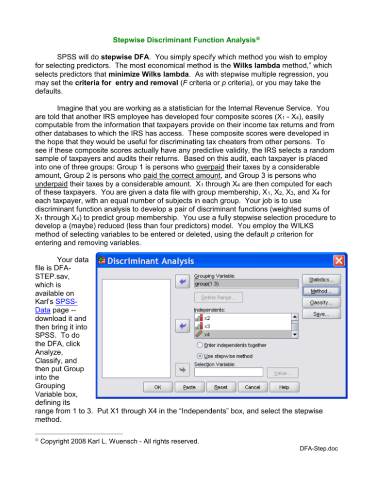
Your data
file is DFASTEP.sav,
which is
available on
Karl’s SPSSData page -download it and
then bring it into
SPSS. To do
the DFA, click
Analyze,
Classify, and
then put Group
into the
Grouping
Variable box,
defining its
range from 1 to 3. Put X1 through X4 in the “Independents” box, and select the stepwise
method.

Copyright 2008 Karl L. Wuensch - All rights reserved.
DFA-Step.doc
Page 2
Click Method and select “Wilks’ lambda” and “Use probability of F.” Click Continue.
Under Statistics, ask for the group means. Under Classify, ask for a territorial map.
Continue, OK.
Look at the output, “Variables Not in the Analysis.” At Step 0 the tax groups (overpaid,
paid correct, underpaid) differ most on X3 ( drops to .636 if X3 is entered) and “Sig. of F to
enter” is less than .05, so that predictor is entered first. After entering X3, all remaining
predictors are eligible for entry, but X1 most reduces lambda, so it enters. The Wilks lambda
is reduced from .635 to .171. On the next step, only X 2 is eligible to enter, and it does,
lowering Wilks lambda to .058. At this point no variable already in meets the criterion for
removal and no variable out meets the criterion for entry, so the analysis stops.
Look back at the Step 0 statistics. Only X2 and X3 were eligible for entry. Note,
however, that after X3 was entered, the p to enter dropped for all remaining predictors. Why?
X3 must suppress irrelevant variance in the other predictors (and vice versa). After X1 is
added to X3, p to enter for X4 rises, indicating redundancy of X4 with X1.
Interpretation of the Output from the Example Program
If you look at the standardized coefficients and loadings you will see that high
scores on DF1 result from high X3 and low X1. If you look back at the group means you will
see that those who underpaid are characterized by having low X3 and high X1, and thus low
DF1. This suggests that DF1 is good for discriminating the cheaters (those who underpaid)
from the others. The centroids confirm this.
If you look at the standardized coefficients and loadings for DF2 you will see that high
DF2 scores come from having high X2 and low X1. From the group means you see that those
Page 3
who overpaid will have low DF2 (since they have a low X2 and a high X1). DF2 seems to be
good for separating those who overpaid from the others, as confirmed by the centroids for
DF2.
In the territorial map the underpayers are on the left, having a low DF1 (high X1 and
low X3). The overpayers are on the lower right, having a high DF1 and a low DF2 (low X2,
high X3, high X1). Those who paid the correct amount are in the upper right, having a high
DF1 and a high DF2 (low X1, high X2, high X3).
Copyright 2008 Karl L. Wuensch - All rights reserved.