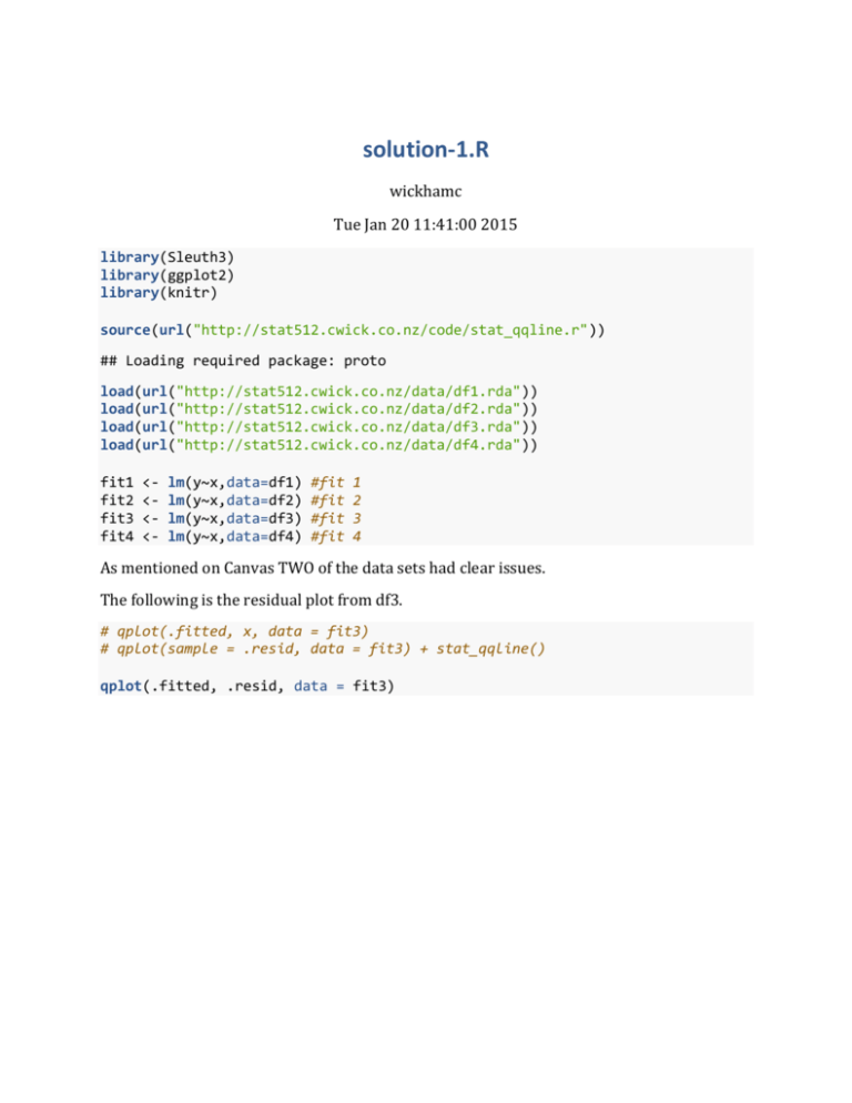
solution-1.R
wickhamc
Tue Jan 20 11:41:00 2015
library(Sleuth3)
library(ggplot2)
library(knitr)
source(url("http://stat512.cwick.co.nz/code/stat_qqline.r"))
## Loading required package: proto
load(url("http://stat512.cwick.co.nz/data/df1.rda"))
load(url("http://stat512.cwick.co.nz/data/df2.rda"))
load(url("http://stat512.cwick.co.nz/data/df3.rda"))
load(url("http://stat512.cwick.co.nz/data/df4.rda"))
fit1
fit2
fit3
fit4
<<<<-
lm(y~x,data=df1)
lm(y~x,data=df2)
lm(y~x,data=df3)
lm(y~x,data=df4)
#fit
#fit
#fit
#fit
1
2
3
4
As mentioned on Canvas TWO of the data sets had clear issues.
The following is the residual plot from df3.
# qplot(.fitted, x, data = fit3)
# qplot(sample = .resid, data = fit3) + stat_qqline()
qplot(.fitted, .resid, data = fit3)
This plot suggests the constant spread (or variation) assumption is violated. Clearly the
spread of the residuals about the zero line decreases as the fitted values increase.
The following is the residual plot from df4.
qplot(.fitted, .resid, data = fit4)
The plot suggests the linearity assumption has be violated as the most residuals are
positive for the ends of the fitted values and negative for middle fitted values.
Interpretation
Since df1 and df2 have no obvious violations the slope and intercept will be interpreted for
both.
First df1
summary(fit1)
##
##
##
##
##
##
##
##
Call:
lm(formula = y ~ x, data = df1)
Residuals:
Min
1Q
-2.2825 -0.8386
Median
0.0814
3Q
0.4580
Max
2.7982
##
##
##
##
##
##
##
##
##
##
Coefficients:
Estimate Std. Error t value Pr(>|t|)
(Intercept)
1.6980
0.2866
5.92 2.2e-06 ***
x
4.0557
0.0566
71.59 < 2e-16 ***
--Signif. codes: 0 '***' 0.001 '**' 0.01 '*' 0.05 '.' 0.1 ' ' 1
Residual standard error: 1.06 on 28 degrees of freedom
Multiple R-squared: 0.995, Adjusted R-squared: 0.994
F-statistic: 5.13e+03 on 1 and 28 DF, p-value: <2e-16
Slope: Is it estimated, that as x increases by 1 unit the mean of y increases by 4.056 units
(corresponding CI (3.940,4.172)).
Intercept: Is it estimated, that when x is equal to zero the mean of y is 1.698 units
(corresponding CI (1.381,2.555)).
For df2
summary(fit2)
##
##
##
##
##
##
##
##
##
##
##
##
##
##
##
##
##
##
Call:
lm(formula = y ~ x, data = df2)
Residuals:
Min
1Q Median
-1.4463 -0.3714 -0.0871
3Q
0.3961
Max
0.8827
Coefficients:
Estimate Std. Error t value Pr(>|t|)
(Intercept)
1.184
0.247
4.79 4.9e-05 ***
x
1.662
0.408
4.07 0.00035 ***
--Signif. codes: 0 '***' 0.001 '**' 0.01 '*' 0.05 '.' 0.1 ' ' 1
Residual standard error: 0.578 on 28 degrees of freedom
Multiple R-squared: 0.372, Adjusted R-squared: 0.349
F-statistic: 16.6 on 1 and 28 DF, p-value: 0.00035
Slope: Is it estimated, that as x increases by 1 unit the mean of y increases by 1.662 units
(corresponding CI (0.825,2.498)).
Intercept: Is it estimated, that when x is equal to zero the mean of y is 1.184 units
(corresponding CI(0.678,1.690)).