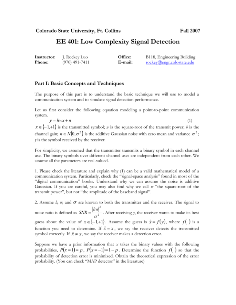
Colorado State University, Ft. Collins
Fall 2007
EE 401: Low Complexity Signal Detection
Instructor:
Phone:
J. Rockey Luo
(970) 491-7411
Office:
E-mail:
B118, Engineering Building
rockey@engr.colostate.edu
Part I: Basic Concepts and Techniques
The purpose of this part is to understand the basic technique we will use to model a
communication system and to simulate signal detection performance.
Let us first consider the following equation modeling a point-to-point communication
system.
y  hwx  n
(1)
x   1,1 is the transmitted symbol; w is the square-root of the transmit power; h is the
channel gain; n  N 0,  2 is the additive Gaussian noise with zero mean and variance  2 ;
y is the symbol received by the receiver.


For simplicity, we assumed that the transmitter transmits a binary symbol in each channel
use. The binary symbols over different channel uses are independent from each other. We
assume all the parameters are real-valued.
1. Please check the literature and explain why (1) can be a valid mathematical model of a
communication system. Particularly, check the “signal-space analysis” found in most of the
“digital communication” books. Understand why we can assume the noise is additive
Gaussian. If you are careful, you may also find why we call w “the square-root of the
transmit power”, but not “the amplitude of the baseband signal”.
2. Assume h, w, and  are known to both the transmitter and the receiver. The signal to
2
hw
noise ratio is defined as SNR  2 . After receiving y, the receiver wants to make its best

guess about the value of x   1,1 . Assume the guess is xˆ  f  y  , where f 

is a
function you need to determine. If xˆ  x , we say the receiver detects the transmitted
symbol correctly. If xˆ  x , we say the receiver makes a detection error.
Suppose we have a prior information that x takes the binary values with the following
probabilities, Px  1  p , Px  1  1  p . Determine the function f   so that the
probability of detection error is minimized. Obtain the theoretical expression of the error
probability. (You can check “MAP detector” in the literature)
3. Use MATLAB to simulate channel uses and detections. This means you will generate x, n,
and compute y. Then you need to compute x̂ from y based on the f   you have derived.
If xˆ  x , you count a detection error. If you do such experiment many times, the number
of error divided by the number of experiments is roughly the probability of detection error.
This is called “Monte-Carlo simulation”. Since the error probability is not computed
theoretically, we say we used Monte-Carlo simulation to estimate the error probability.
Conventionally, we call the number of experiments “the number of Monte-Carlo runs” or
“the number of runs”, “the number of simulations”.
To improve the accuracy of the error probability estimation, you need to make sure the
number of simulations is large enough. Note that the number of simulations depends on
the actual value of the error probability. For example, if error probability is 0.5, 20
simulations can give you a pretty good estimate (close to 0.5). If error probability is 10 4 ,
you will need to set the number of simulations at something around 10 5 .
Try to draw the curve of error probability versus SNR using Monte-Carlo simulations, and
compare the estimated curve with the theoretic curve obtained from the result of step 2.
Suppose the receiver’s prior information about x is not accurate. For example,
Px  1  p , Px  1  1  p , while the receiver believes Px  1  p0  p , and uses
the erroneous prior probability to derive the “optimal” detection function f   . The
detection is therefore suboptimal. Obtain the error probability versus SNR curve using
Monte-Carlo simulation, and compare it with the curve obtained using the optimal detector
(i.e., the f   function derived using the correct Px  1  p ).