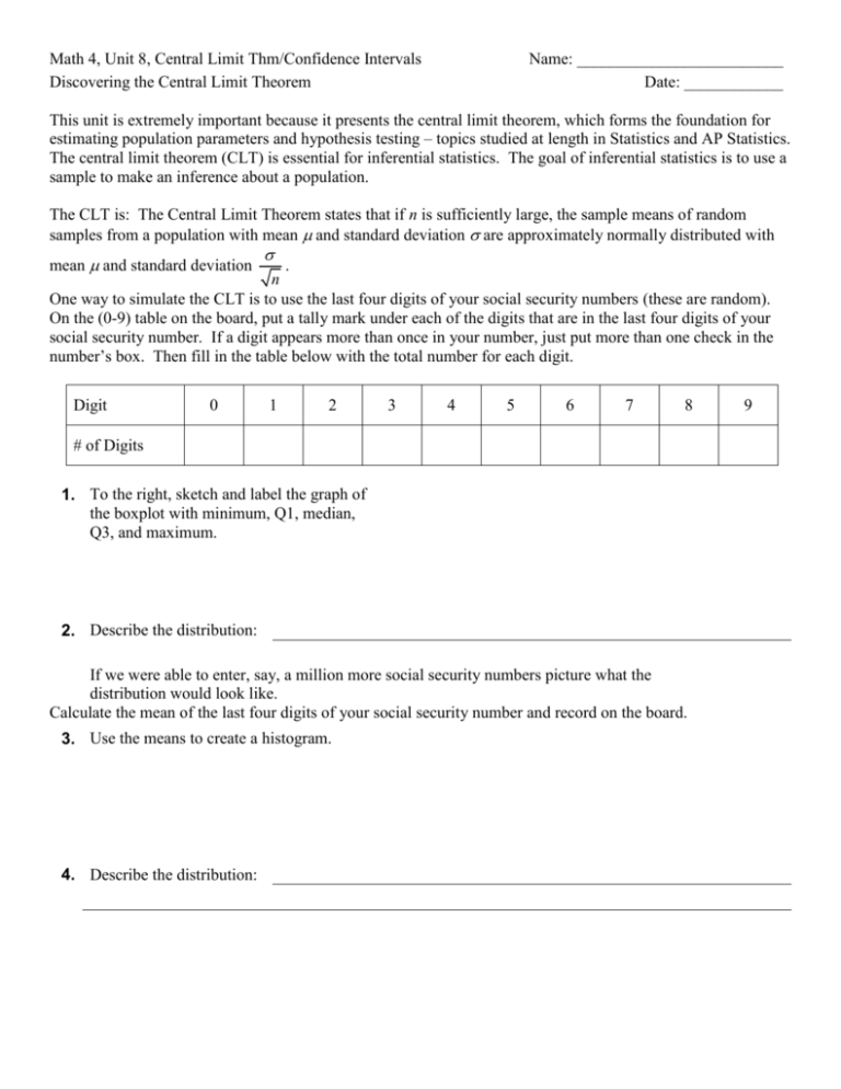
Math 4, Unit 8, Central Limit Thm/Confidence Intervals
Discovering the Central Limit Theorem
Name: _________________________
Date: ____________
This unit is extremely important because it presents the central limit theorem, which forms the foundation for
estimating population parameters and hypothesis testing – topics studied at length in Statistics and AP Statistics.
The central limit theorem (CLT) is essential for inferential statistics. The goal of inferential statistics is to use a
sample to make an inference about a population.
The CLT is: The Central Limit Theorem states that if n is sufficiently large, the sample means of random
samples from a population with mean  and standard deviation  are approximately normally distributed with
mean  and standard deviation

.
n
One way to simulate the CLT is to use the last four digits of your social security numbers (these are random).
On the (0-9) table on the board, put a tally mark under each of the digits that are in the last four digits of your
social security number. If a digit appears more than once in your number, just put more than one check in the
number’s box. Then fill in the table below with the total number for each digit.
Digit
0
1
2
3
4
5
6
7
8
# of Digits
1. To the right, sketch and label the graph of
the boxplot with minimum, Q1, median,
Q3, and maximum.
2. Describe the distribution:
If we were able to enter, say, a million more social security numbers picture what the
distribution would look like.
Calculate the mean of the last four digits of your social security number and record on the board.
3. Use the means to create a histogram.
4. Describe the distribution:
9
One key element of the central limit theorem tells us: if the sample size is large enough, the distribution of
sample means can be approximated by a normal distribution, even if the original population is not
normally distributed.
5. Find the mean and standard deviation of the data in the table.
What is the theoretical mean & standard deviation?
Compare these values to the CLT values (remember,  x =

n
).
The Central Limit Theorem and the Sampling Distribution of x
Given:
1. The random variable x has a distribution (which may or may not be normal) with mean  and
standard deviation .
2. Simple random samples all of the same size n are selected from the population.
Conclusions:
1. The distribution of sample means x will, as the sample size increases, approach a normal
distribution.
2. The mean of all sample means is the population mean . (i.e. the normal distribution from
conclusion 1 has mean .)
3. The standard deviation of all sample means is
conclusion 1 has standard deviation

n

n
. (i.e. the normal distribution from
.)
Practical Rules Commonly Used:
1. If the original population is not itself normally distributed, here is a common guideline: For
samples of size n greater than 30, can be approximated reasonably well by a normal
distribution. (There are rare exceptions.) As n gets larger, the approximation gets better.
2. If the original population is normally distributed, then (of course) the sample means will be
normally distributed (n can be any value).
Common Notations:
As you know, we use for mean of populations. We use  x for mean of the sample means.
We use (you guessed it)  x for the standard deviation of the sample means.
So our formulas are:  x   and  x 

n
.  x is often called standard error of the mean.
EXAMPLE: The Sky Lift at Six Flags carries
patrons from one end of the park to the other. The
car, called a gondola, bears a plaque stating that
the maximum capacity is 12 people or 2004
pounds. Because men tend to weigh more than
women, a “worse case” scenario involves 12
passengers who are all men. Men have weights
that are normally distributed with a mean of 172
lb. and standard deviation of 29 lb.
a)
Find the probability that if an individual man is randomly selected, his weight will be
greater than 167. (why 167?) (this is an old z-score problem)
b)
Find the probability that 12 randomly selected men will have a mean greater than 167.
EXERCISES:
For items 1 – 3, use the example problem.
1. If 36 men are randomly selected, find the probability that they have a mean weight less than 167.
2. If 64 men are randomly selected, find the probability that they will have a mean weight between
170 and 175.
3. a)
b)
If 25 men are randomly selected, find the probability that they will have a mean weight
between 160 and 180.
Why can the central limit theorem be used in part (a), even though the sample size does not
exceed 30?
4. Assume that cans of Soda are filled so that the actual amounts have a mean of 12.00 oz.
and a standard deviation of 0.11 oz.
a) Find the probability that a sample of 36 cans will have a mean amount of at
least 12.05 oz.
b) Based from the result in part (a), is it reasonable to believe that the cans are
actually filled with a mean of 12 oz? If the mean is not 12 oz, are customers
being cheated?
5. The manager of an electronics store is concerned that his suppliers have been selling him
TV sets with lower than average quality. Research shows that replacement times for TV
sets have a mean of 8.2 years and a standard deviation of 1.1 years. He randomly selects
50 of the TV sets that he sold and finds that the mean replacement time was 7.8 years.
a) Find the probability that 50 randomly selected TV sets will have a mean
replacement time of 7.8 years or less.
b) Based from the result in part (a), does it appear that the electronics company has
been selling TV sets that have lower than average quality?
6. Scores for men on the SAT verbal portion are normally distributed with a mean of 509
and a standard deviation of 112.
a) If 16 men take the test, find the probability that the mean of these 16 is 590 or
more.
b) If those 16 had taken a course to improve verbal SAT scores, is there evidence
that the course was effective?