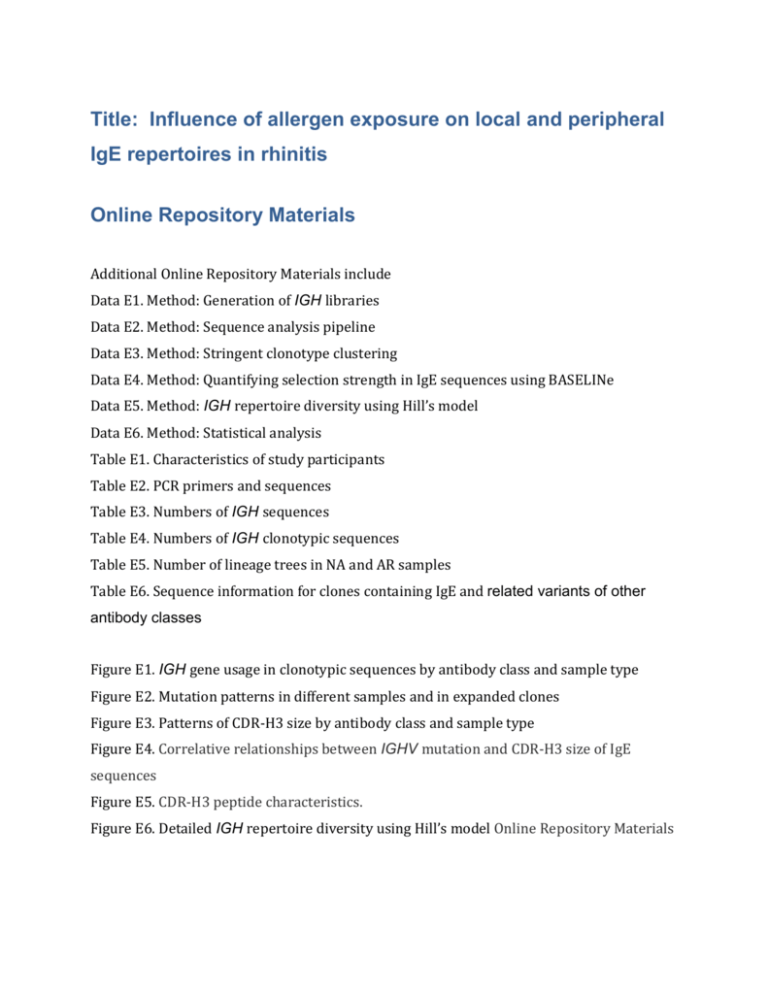
Title: Influence of allergen exposure on local and peripheral
IgE repertoires in rhinitis
Online Repository Materials
Additional Online Repository Materials include
Data E1. Method: Generation of IGH libraries
Data E2. Method: Sequence analysis pipeline
Data E3. Method: Stringent clonotype clustering
Data E4. Method: Quantifying selection strength in IgE sequences using BASELINe
Data E5. Method: IGH repertoire diversity using Hill’s model
Data E6. Method: Statistical analysis
Table E1. Characteristics of study participants
Table E2. PCR primers and sequences
Table E3. Numbers of IGH sequences
Table E4. Numbers of IGH clonotypic sequences
Table E5. Number of lineage trees in NA and AR samples
Table E6. Sequence information for clones containing IgE and related variants of other
antibody classes
Figure E1. IGH gene usage in clonotypic sequences by antibody class and sample type
Figure E2. Mutation patterns in different samples and in expanded clones
Figure E3. Patterns of CDR-H3 size by antibody class and sample type
Figure E4. Correlative relationships between IGHV mutation and CDR-H3 size of IgE
sequences
Figure E5. CDR-H3 peptide characteristics.
Figure E6. Detailed IGH repertoire diversity using Hill’s model Online Repository Materials
Data E1 Method: generation of IGH libraries
IGH genes were amplified from cDNA in semi-nested PCR reactions, with minor changes of
previously reported methods (E1). In brief, PCR1 reaction mix (20μl) consisted of 2 μl
cDNA, 200 μM each dNTP (Promega, UK), 0.4U Phusion DNA polymerase (NEB, UK), six
FW1/IGHV gene family primers (41.75 nM each) in conjunction with constant region
primers (either IGα-1, IGγ-1, IGε-1, or IGμ-1; 250 nM; Table E2). Subsequently, reamplification from 2.5 μl PCR1 products were performed in PCR2 reaction mix (25 μl),
comprising 200 μM each dNTP, 0.5 U Phusion DNA polymerase and six FW1/IGHV gene
family primers (41.75 nM each) in combination with antibody class specific, nested
constant region primers (IGα-2, IGγ-2, IGε-2, or IGμ-2; 250 nM) where all primers were
labeled at the 5’-end with Multiplex Identifiers (MIDs) for multiplexing of twelve different
libraries. PCR thermal cycling is as follows: 98°C for (30 s), 25(PCR1), or (PCR2) cycles of
98°C (10 s); 60°C (15 s); 72°C (45 s), and 1 cycle of 72°C (5 min). To produce sufficient
amounts of amplicons for pyrosequencing on the 454 GS FLX+ System, eight different PCR1
reactions per sample, followed by two PCR2 reactions (16 reactions in total per sample)
were performed for each class, which were then purified from 1.5% TAE agarose gels using
the Silica Bead Gel Purification Kit (Thermo Scientific, UK). Amplicons from 16 reactions
and four classes were combined as one library (using the same MID barcode), and further
enriched using the QIAquick PCR Purification Kit (Qiagen, UK).
Data E2 Method: Sequence analysis pipeline
This was performed as previously described (E2) but with extensions to include IgE
sequences. In the initial quality control step a range of criteria are used to identify and then
exclude artefactual sequences that may have arisen as a consequence of PCR or Online
Repository Materials Wu et al. 3 ligation errors, as well as a more general requirement to
meet various markers of biological plausibility based on known information about the
germline sequence.
Sequences that pass quality control are then annotated using IMGT/HighV-QUEST (E3) and
the output files parsed into a single table. The nucleotide sequences for the defined CDR-H3
regions were then used to compare all sequences in a pairwise fashion. For each pairwise
comparison the minimum nucleotide edit distance (including indels) between CDR-H3s
was calculated and standardised to the shorter of the two CDR-H3 regions. In those cases
where the standardised edit distance was greater than 0.2, or where IGHV gene identity
was called for both sequences by IMGT HighV-QUEST and those IGHV genes did not match,
then the edit distance was set to 1. This forces those two sequences to be in separate
clusters, and also ensures that all members of a cluster have the same IGHV gene. This
distance matrix was then subjected to hierarchical clustering (complete linkage) and the
subsequent dendrogram was cut at a defined height so as to generate the final clusters
(clones). Finally, for each cluster an exemplar sequence was chosen to represent that clone
in downstream analysis. These were determined predominantly on the basis of being the
modal sequence in the cluster, but also with some weight given to IGHJ family usage (so as
to generate an exemplar sequence that illustrated the most common sequence and IGHJ
family usage). All analyses before and after IMGT/HighV-Quest were performed in R (E4)
using custom scripts. The background error frequency for the whole system was
approximately 2% (E2).
Data E3. Method: Stringent clonotype clustering
Prior to analysis of selection strength, diversity and lineage, more stringent clustering
criteria were imposed on QC-filtered sequence data. First, an initial "preclone" categorical
grouping required sequences to share the same clonotypic characteristics (the same IGHV
genes, IGHJ genes and CDR-H3 junction length). A second step that further divided
"preclones" into clones based on a within-clone junctional nucleotide distance of 5.
Distance was measured as the number of point mutations weighted by a symmetric version
of the nucleotide substitution probability previously described (E5).
Data E4. Method: Quantifying selection strength in IgE sequences using
BASELINe
Selection strength was estimated as previously described (E6) with the Focused test
statistic and S5F mutation model (E7). In brief, BASELINe quantifies selection strength (Σ)
as the log-odds ratio between the observed and expected replacement frequencies. The
expected frequencies are calculated using the S5F model to account for SHM hot/cold-spots
and substitution preferences. Rather than a single point estimate for the selection strength,
BASELINe utilizes a Bayesian framework to compute the complete probability density for
Σ, thus providing a quantification of uncertainty in the analysis. Positive Σ values indicate
an increased frequency of replacements (positive selection), while negative Σ values
indicate a decreased frequency (negative selection) relative to a background model of SHM.
Data E5. Method: IGH repertoire diversity using Hill’s model
The repertoire diversity was analysed using the method proposed by Hill (E8). This
method quantifies diversity as a smooth function (qD) of a single parameter (q):
where S is the number of clones, pi is the proportional abundance of the ith clone and the
parameter q determines how clonal frequencies are weighted. Special cases of this general
index of diversity correspond to the most popular diversity measures in ecology: species
richness (q = 0), the exponential Shannon–Weiner index (q = 1), and the inverse of the
Simpson index (q = 2).
At q=0 different species weight equally, regardless of their abundance or rarity within the
population and this total clonal diversity (0D) is illustrated in Figure 5. In general, as the
parameter q varies from 0 to +∞ the diversity number (qD) depends less on rare species
and more on common (abundant) ones, thus encompassing a range of definitions that can
be visualized as a single curve (Fig E6). For example in Figure E6, A, as q values increased,
the IgE diversity was similar to that of IgG and IgM in the blood (i.e. it was no more
dominated by a single clone). In contrast, IgA in the blood tended to be more dominated by
a single clone. This full curve contains significantly more information than any single
measure, and is thus preferable to the approaches used in most existing studies. To account
for differences in sequencing depth, the number of sequences in each diversity calculation
was set to the minimum across groups through repeated sub--‐sampling with
replacement. Confidence intervals were constructed using the percentile method and a
95% confidence interval for each qD was determined via bootstrapping (2,000
permutations).
Data E6. Method: Statistical analysis
Different statistical approaches were used to compare groups in each figure.
Figure 1, A; Figure E1, A & B: χ2 test with Sidak adjustment using the absolute count of
clonotypes by IGHV family usage pooled from multiple individuals.
Figure 1, B & C; Figure E1, C-F: RM one-way ANOVA with the Greenhouse-Geisser correct
(parametric, paired) with Holm-Sidak’s multiple comparisons test using the relative
frequency derived from the absolute count of clonotypes by gene usage within individuals
for comparison between antibody classes.
Figure E1, G-J: Ordinary one-way ANOVA (parametric, unpaired) with Holm-Sidak’s
multiple comparisons tests using the relative frequency derived from the absolute count of
clonotypes by gene usage within individuals for comparison between antibody classes.
Figure 2, A & B; Figure 3, B-D; Figure E2, A, B, D, E; Figure E3 B & C; Figure E5: KruskalWallis test (non-parametric, unpaired), with Dunn's post-test for multiple comparisons.
Figure 2, C - F: Mann-Whitney test (non-parametric, unpaired).
Figure 5: P-values for comparing the diversities of two groups (a and b) were generated
via bootstrap of Δ0D, the difference between the estimated diversity in each group. Each
bootstrap realization i is generated by resampling (with replacement) equivalent numbers
of sequences from groups a and b, and calculating:
where B=2,000 is the number of bootstrap realizations, and
is the diversity score at q=0 (Data 5) for group g. For each comparison, group a is defined
by having the higher median diversity compared with group b. The p-value is then
calculated using the percentile method and doubled to account for the two-tailed nature of
the test.
Figure 6: Focused test statistic and S5F mutation model.