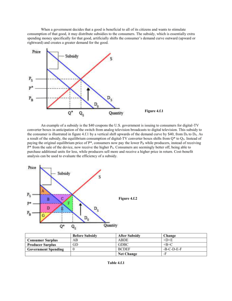
When a government decides that a good is beneficial to all of its citizens and wants to stimulate
consumption of that good, it may distribute subsidies to the consumers. The subsidy, which is essentially extra
spending money specifically for that good, artificially shifts the consumer’s demand curve outward (upward or
rightward) and creates a greater demand for the good.
Figure 4.f.1
An example of a subsidy is the $40 coupons the U.S. government is issuing to consumers for digital-TV
converter boxes in anticipation of the switch from analog television broadcasts to digital television. This subsidy to
the consumer is illustrated in figure 4.f.1 by a vertical shift upwards of the demand curve by $40, from D0 to DS. As
a result of the subsidy, the equilibrium consumption of digital-TV converter boxes shifts from Q* to Q S. Instead of
paying the original equilibrium price of P*, consumers now pay the lower PB while producers, instead of receiving
P* from the sale of the device, now receive the higher PS. Consumers are seemingly better off, being able to
purchase additional units for less, while producers sell more and receive a higher price in return. Cost-benefit
analysis can be used to evaluate the efficiency of a subsidy.
Figure 4.f.2
Consumer Surplus
Producer Surplus
Government Spending
Before Subsidy
AB
GD
0
After Subsidy
ABDE
GDBC
BCDEF
Net Change
Table 4.f.1
Change
+D+E
+B+C
-B-C-D-E-F
-F
From the cost-benefit analysis in table 4.f.1, we see that consumers gain areas D and E in consumer
surplus. Similarly, producers gain areas B and C in producer surplus. Judging based on consumers and producers
alone, it seems as though subsidies are beneficial overall. However, when we consider the expense for the
government to provide the subsidy, represented by area BCDEF, we find that there is a dead-weight loss of area F to
the economy.
A subsidy is not always granted to consumers. For example, the government may feel that steel is an
important commodity and subsidize steel producers to stimulate production.
Figure 4.f.3
Subsidy = $4/unit
The subsidy to the producer is viewed as a decrease in production costs, which allows producers to expand
production from S0 to SS. In figure 4.f.3, the vertical distance between the original supply curve and the subsidized
supply curve again represents the subsidy provided by the government. In this case, the subsidy is $4, calculated as
$10 - $6. The result of the subsidy is increased production, from an equilibrium quantity of 10 to 13, which is
matched by increased consumption by consumers. Consumers now pay $6 instead of the equilibrium $9, and
producers receive $10 instead of $9.
This graph also illustrates another point that relates subsidies to the elasticity of the supply or demand
curve. In this particular example, the supply curve is much more elastic than previous examples. Due to the flatness
of the curve, the supplier receives less of the subsidy, represented by region A, than consumers, represented by area
B. The amount of producer surplus can be calculated by using the area formula of a trapezoid, which is the average
of its bases times the height. The area enclosed by region A represents $11.50 [Calculated as
]. The consumer surplus, region B, on the other hand, represents $34.50 [Calculated as
]. The entire cost of the subsidy is the sum of area ABC, or $52 [Calculated as
], which means that the remaining dead-weight loss, area C, must equal $6 [Calculated as
]. It becomes apparent that the flatter the curve of the supplier, the less of the subsidy they receive.
The opposite is also true of demanders – the flatter their demand curve, the less subsidy they would receive. If a
curve was perfectly elastic, then any subsidy would go entirely to the other party (i.e., if the supply curve was
perfectly elastic, or flat, then the entire amount of the subsidy will fall solely into the hands of the consumers).