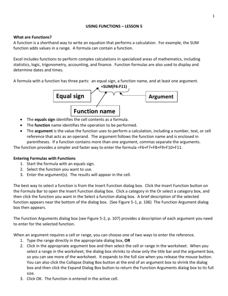
1
USING FUNCTIONS – LESSON 5
What are Functions?
A function is a shorthand way to write an equation that performs a calculation. For example, the SUM
function adds values in a range. A formula can contain a function.
Excel includes functions to perform complex calculations in specialized areas of mathematics, including
statistics, logic, trigonometry, accounting, and finance. Function formulas are also used to display and
determine dates and times.
A formula with a function has three parts: an equal sign, a function name, and at least one argument.
=SUM(F6:F11)
Equal sign
Argument
Function name



The equals sign identifies the cell contents as a formula.
The function name identifies the operation to be performed.
The argument is the value the function uses to perform a calculation, including a number, text, or cell
reference that acts as an operand. The argument follows the function name and is enclosed in
parentheses. If a function contains more than one argument, commas separate the arguments.
The function provides a simpler and faster way to enter the formula =F6+F7+F8+F9+F10+F11.
Entering Formulas with Functions
1. Start the formula with an equals sign.
2. Select the function you want to use.
3. Enter the argument(s). The results will appear in the cell.
The best way to select a function is from the Insert Function dialog box. Click the Insert Function button on
the Formula Bar to open the Insert Function dialog box. Click a category in the Or select a category box, and
then click the function you want in the Select a function dialog box. A brief description of the selected
function appears near the bottom of the dialog box. (See Figure 5-1, p. 106) The Function Argument dialog
box then appears.
The Function Arguments dialog box (see Figure 5-2, p. 107) provides a description of each argument you need
to enter for the selected function.
When an argument requires a cell or range, you can choose one of two ways to enter the reference.
1. Type the range directly in the appropriate dialog box, OR
2. Click in the appropriate argument box and then select the cell or range in the worksheet. When you
select a range in the worksheet, the dialog box shrinks to show only the title bar and the argument box,
so you can see more of the worksheet. It expands to the full size when you release the mouse button.
You can also click the Collapse Dialog Box button at the end of an argument box to shrink the dialog
box and then click the Expand Dialog Box button to return the Function Arguments dialog box to its full
size.
3. Click OK. The function is entered in the active cell.
2
Entering a Function Directly in a Cell Using Formula AutoComplete
Formula AutoComplete helps you enter a formula with a valid function name and arguments (see Figure 5-3,
p. 108). As you begin to type the function name, a list of function names appears below the active cell. The
functions listed match the letter you have typed. Continue typing until you see the function you want. Then
double-click the name of the function you want. The function and its arguments appear in a ScreenTip below
the cell. You can use the ScreenTip as a guide to enter the necessary arguments.
Step-by-Step 5.1 (p. 108)
Types of Functions
Mathematical and Trigonometric Functions – are used to manipulate quantitative data in a worksheet.
Some mathematical operations, such as, addition, subtraction, multiplication, and division, do not
require functions.
However, mathematical and trigonometric functions are particularly useful when you need to
determine values such as logarithms, factorials, sines, cosines, tangents, and absolute values.
FUNCTION
SQRT (number)
ROUND(number, num_digits)
LN (number)
RETURNS
The square root of the number in the argument. For
example, =SQRT(C4) returns the square root of the value in
cell C4.
The number in the first argument rounded to the number
of decimal places designated in the second argument. For
example, =ROUND(14.23444, 2) returns 14.23, which
rounds the number in the first argument to two decimal
places. If the second argument is a negative number, the
first argument is rounded to the left of the decimal point.
For example, =ROUND(142.3433, -2) returns 100.
The natural logarithm of a number. For example, =LN(50)
returns 1.69897.
Step-by-Step 5.2 (p. 110)
Statistical Functions—are used to describe large quantities of data. For example, average, standard
deviation, or variance of a range of data. Statistical functions can also determine the number of values
in a range, the largest value in a range, and the smallest value in a range. All the statistical functions
contain a range for the argument. You can include multiple ranges by entering additional arguments.
The range is the body of numbers the statistics will describe.
FUNCTION
RETURNS
AVERAGE(number1, number2 . . .)
The average (or man) of the range; for example,
=AVERAGE(E4:E9) returns the average of the
numbers in the range A4:E9
COUNT(value1, value2. . . )
The number of cells in the range that contain
numbers; for example, =COUNT(D6:D21) returns
16 if all the cells in the range contain numbers
3
COUNTA(value1, value2. . .)
MAX(number1, number2. . . )
MIN(number1, number 2 . . .)
STDEV (number1, number2 . . .)
VAR(number1, number2 . . .)
The number of cells in the range that contain
data; for example =COUNT(B4:B15) returns 11 if
all the cells I the range contain data
The largest number in the range
The smallest number I the range
The estimated standard deviation of the numbers
in the range
The estimated variance of the numbers in the
range
Step-by-Step 5.3 (p. 112)
Financial Functions—are used to analyze loans and investments. The primary functions are future
value, present value, and payment. Note that for these functions to return the correct value, the
payment and the interest rate must have the same time period. For example, the payment period is
usually expressed in months, whereas the interest rates are commonly expressed in years. So, it the
payment period is monthly, you must divide the annual interest by 12 to determine the monthly rate.
FUNCTION
FV(rate, nper, pmt, pv, type)
PV(rate, nper, pmt, fv, type)
PMT(rate,nper,pv,fv,type)
RETURNS
The future value of an investment based on equal
payments (third argument), at a fixed interest rate (first
argument), for a specified number of periods (second
argument). (The fourth and fifth arguments for the
present value of the investment and the timing of the
payments are optional.) For example, =FV(.08,5,100)
determines the future value of five $100 payments
earning an 8% interest rate at the end of five years.
The present value of a loan or an investment based on
equal payments (third argument), at a fixed interest rate
(first argument), for a specified number of payments
(second argument). (The fourth and fifth arguments for
the future value of the investment and the timing of the
payments are optional.) For example, =PV(.1,5,500)
displays the current value of five payments of $500 at a
10% interest rate.
The equal payments needed to repay a loan (third
argument), at a fixed interest rate (first argument), in a
specified number of periods (second argument). (The
fourth and fifth arguments for the future value of the
loan and the timing of the payments are optional.) For
example, =PMT(.01,36,10000) displays the monthly
payment needed to repay a $10,000 loan at a 1%
monthly interest rate (12% annual interest rate divided
by 12 months) for 36 months (three years divided by 12
months).
4
Step-by-Step 5.4 (p. 115)
Logical Functions
Logical functions, such as the IF function, display text or values if certain conditions exist.
In the IF function,
1. The first argument sets a condition for comparison, called a logical test.
2. The second argument determines the value that appears in the cell if the logical test is true.
3. The third argument determines the value that appears in the cell if the logical test is false.
For example, a teacher might use the IF function to determine whether a student has passed or failed a
course. The formula =IF(C4>60, “PASS”, “FAIL”) returns PASS if the value in cell C4 is greater than 60. The
formula returns FAIL if the value in cell C4 is not greater than 60.
FUNCTION
IF(logical_test,
value_if_true,value_if_false)
RETURNS
One value if the condition in the logical test is true, and
another value if the condition I the logical test is false; for
example, =IF(2+2=4, Over, Under) returns Over
AND(logical1, logical2, . . .)
TRUE if all of the arguments are true, and FALSE if any or
all of the arguments are false; for example,
=AND(1+1=2,1+2=3) returns TRUE, and
=AND(1+1=2,1+2=4) returns FALSE
OR(logical1,logical2, . . .)
TRUE if any of the arguments are true, and FALSE if none
of the arguments is true; for example,
=OR(1+1=2,1+2=3) returns TRUE, and
=OR(1+1=2,1+2=4) returns TRUE, but
=OR(1+1=3,1+2=4) returns FALSE
NOT(logical)
TRUE if any of the arguments are true, and FALSE if the
argument is true; for example, =NOT(2+2=4) returns
TRUE, but =NOT(2+2=4) returns FALSE
IFERROR(value,value_if_error) The formula results if the first argument contains no
error, and the specified value if the argument is incorrect;
for example, =IFERROR(2+2=1, “Error in calculation”)
returns Error in calculation
Step-by-Step 5.5 (p. 117)
Date and Time Functions
Functions can be used to insert dates and times in a worksheet. For example, date and time functions can be
used to convert serial numbers to a month, a day, or a year. A date function can also be used to insert the
current date or the current date and time.
FUNCTION
RETURNS
DATE(year,month,day) The date specified in the year, month, and day arguments,
which are entered as numbers. For example,
=DATE(2010,5,23) returns 5/23/2010
NOW()
The current date and time based on the computer’s date and
5
TODAY()
time settings. For example, =NOW() returns the current date
and time, such as 5/23/2010 22:05. This function has no
arguments.
The current date based o the computer’s date setting and
formatted as a date. For example, = TODAY() returns the
current date, such as 5/23/2010. This function has no
arguments.
Text Functions
Text functions are used to format and work with cell contents. A text function can be used to convert text in a
cell to all uppercase or lowercase letters. Text functions can also be used to repeat data contained in another
cell.
FUNCTION
PROPER()
OPERATION
Converts the first letter of each word in the
specified cell to uppercase and the rest to
lowercase.
LOWER()
Converts all letters in the specified cell to
lowercase.
UPPER()
Converts all letters in the specified cell to
uppercase.
SUBSTITUTE(text,old_text,new_text,instance_num) Replaces existing text (the second
argument) in a specified cell (the first
argument) with new text (third argument).
If you omit the optional fourth argument,
instance_num, every occurrence of the text
is replaced. For example, =SUBSTITUTE(C2,
“Income”, “Revenue”) replaces every
instance of the word Income in cell C2 with
the word Revenue.
REPT(text,number_times)
Repeats the text (first argument) in the
specified cell a specified number of times
(second argument). For example,
=REPT(B6,3) repeats the text in cell B6 three
times.
Step-by-Step 5.6 (p. 120)