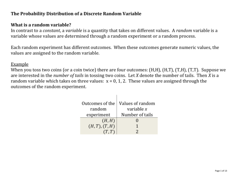
The Probability Distribution of a Discrete Random Variable
What is a random variable?
In contrast to a constant, a variable is a quantity that takes on different values. A random variable is a
variable whose values are determined through a random experiment or a random process.
Each random experiment has different outcomes. When these outcomes generate numeric values, the
values are assigned to the random variable.
Example
When you toss two coins (or a coin twice) there are four outcomes: (H,H), (H,T), (T,H), (T,T). Suppose we
are interested in the number of tails in tossing two coins. Let X denote the number of tails. Then X is a
random variable which takes on three values: x = 0, 1, 2. These values are assigned through the
outcomes of the random experiment.
Outcomes of the Values of random
random
variable x
experiment
Number of tails
(𝐻, 𝐻)
0
(𝐻, 𝑇), (𝑇, 𝐻)
1
(𝑇, 𝑇)
2
Page 1 of 13
Example
When you guess the answer to a multiple choice question, you are conducting a random experiment. The
outcomes are, you are either correct or incorrect. If a quiz has five multiple choice questions and you
guess the answers for all five, you are conducting a random experiment which consists of five identical
trials. Each trial has two outcomes. Since there are five trials, then the total number of outcomes is
25 = 32. Now, let 𝑋 be the random variable denoting the number of correct guesses. The outcomes of this
random experiment and values generated and assigned to the random variable 𝑋 are shown below. For
ease of presentation, “0” represents “incorrect” and “1” is for a “correct” guess. For example, the outcome
(0,0,0,0,0) represent all incorrect guesses.
Outcomes of the random experiment (0 = Incorrect guess; 1 = Correct guess)
(0,0,0,0,0)
(1,0,0,0,0), (0,1,0,0,0), (0,0,1,0,0), (0,0,0,1,0), (0,0,0,0,1)
(1,1,0,0,0), (1,0,1,0,0), (1,0,0,1,0), (1,0,0,0,1), (0,1,1,0,0), (0,1,0,1,0), (0,1,0,0,1), (0,0,1,1,0), (0,0,1,0,1), (0,0,0,1,1)
(1,1,1,0,0), (1,1,0,1,0), (1,1,0,0,1), (1,0,1,1,0), (1,0,1,0,1), (1,0,0,1,1), (0,1,1,1,0), (0,1,1,0,1), (0,1,0,1,1), (0,0,1,1,1)
(1,1,1,1,0), (1,1,1,0,1), (1,1,0,1,1), (1,0,1,1,0), (0,1,1,1,1)
(1,1,1,1,1)
𝑥
Correct guesses
0
1
2
3
4
5
Page 2 of 13
Probability Distribution of a Discrete Random Variable
What makes 𝑋 a random variable is that, although we know the different values it can take on, its specific
value is not known until we conduct the random experiment. For discrete (versus continuous) random
variables, all possible values of the random variable can be listed. Furthermore, each value of the
discrete random variable has a distinct probability of occurring. Thus, if we list all possible values of a
discrete random variable and the corresponding probability of each value, then we have a probability
distribution of that discrete random variable.
Example
Let 𝑋 be the random variable denoting the number of tails when tossing two coins. Let 𝑥𝑖 denote the
values and 𝑓(𝑥𝑖 ) the probability of each value. The probability distribution of 𝑋 is:
Outcomes
(𝐻, 𝐻)
(𝐻, 𝑇), (𝑇, 𝐻)
(𝑇, 𝑇)
𝑥𝑖
0
1
2
𝑓(𝑥𝑖 )
0.25
0.50
0.25
1.00
Page 3 of 13
Example
A company employs salespersons to market its product. Keeping track of sales for 100 weeks, the
following table shows the number of units of the product sold per week and the frequency of the weeks.
For example, in 15 of the weeks, a salesperson sold 11 units, and in 40 of the weeks, 12 units were sold.
Number of units sold Weeks
x
Frequency
10
10
11
15
12
40
13
30
14
5
100
Using this table, we can generate the probability (relative frequency) distribution of the random
variable 𝑋 (the number of units sold in a given week), as shown below.
Probability Distribution of 𝑋
Number of items sold Probability
𝑓(𝑥)
𝑥
10
0.10
11
0.15
12
0.40
13
0.30
14
0.05
1.00
Page 4 of 13
Expected Value of a Random Variable
The expected value of x, denoted by 𝐄(𝒙), is the weighted mean of 𝑥 values. The weights are the
probability of each value of the random variable.
In the previous chapter the formula for the weighted mean was: µ = 𝑥𝑖 𝑤𝑖 .
To find the expected value of the random variable X, just replace 𝑤𝑖 with 𝑓(𝑥𝑖 ):
E(𝑥) ≡ µ = 𝑥𝑖 𝑓(𝑥𝑖 )
Example
Find the expected value of the number of units sold per week in the previous example.
𝑥𝑖
10
11
12
13
14
𝑓(𝑥𝑖 )
0.10
0.15
0.40
0.30
0.05
𝑥𝑖 𝑓(𝑥𝑖 )
1.00
1.65
4.80
3.90
0.70
12.05
E(𝑥 ) ≡ µ = 𝑥𝑖 𝑓(𝑥𝑖 ) = 12.05
This means that the mean weekly sales is 12.05 units.
Page 5 of 13
Variance of a Random Variable
The variance of X is the measure of dispersion of 𝑥𝑖 about the center of gravity µ = E(𝑥𝑖 ). The variance of
a random variable is the expected value or the (weighted) mean of the squared deviations (𝑥 − µ)2
var(𝑥) = E[(𝑥 − µ)2 ] = (𝑥 − µ)2 𝑓(𝑥)
To find the weighted mean of (𝑥 − µ)2 multiply each squared deviation by the corresponding weight 𝑓(𝑥)
and the sum the products.
Example
Find the variance of the number of units sold per week in the previous example.
𝑥
10
11
12
13
14
𝑓(𝑥)
0.10
0.15
0.40
0.30
0.05
(𝑥 − µ)2
4.2025
1.1025
0.0025
0.9025
3.8025
(𝑥 − µ)2 𝑓(𝑥)
0.4203
0.1654
0.0010
0.2708
0.1901
1.0475
𝐸 (𝑥 ) = 12.05
var(𝑥) = (𝑥 − µ)2 𝑓(𝑥) = 1.0475
sd(𝑥) = √var(𝑥) = 1.0235
Page 6 of 13
Computational Formula for 𝐯𝐚𝐫(𝒙)
Just a simple derivation!
var(𝑥) = E(𝑥 2 ) − µ2
var(𝑥) = 𝑥 2 𝑓(𝑥) − µ2
𝑥
10
11
12
13
14
𝑓(𝑥)
0.10
0.15
0.40
0.30
0.05
𝑥 2 𝑓(𝑥)
10.00
18.15
57.60
50.70
9.80
146.25
var(𝑥 ) = 146.25 − 12.052 = 1.0475
Page 7 of 13
Arithmetic Properties Of Expected Value And Variance
The arithmetic properties of E(x) and var(𝑥) shows what happens to the expected value and variance of x
if the random variable is linearly transformed. The random variable Y is a linear transformation of X, if
for any constant a and a nonzero constant b,
𝑦 = 𝑎 + 𝑏𝑥
Then for any linear transformation of X, the following holds:
1. 𝐸(𝑦) = 𝑎 + 𝑏𝐸(𝑥)
𝑦 = 𝑎 + 𝑏𝑥
E(𝑦) = E(𝑎 + 𝑏𝑥)
E(𝑦) = 𝐸 (𝑎) + 𝐸(𝑏𝑥)
E(𝑦) = 𝑎 + 𝑏𝐸(𝑥)
2. var(𝑦) = 𝑏 2 var(𝑥 )
var(𝑦) = var(𝑎 + 𝑏𝑥)
var(𝑦) = var(𝑎) + var(𝑏𝑥)
var(𝑦) = 𝑏 2 var(𝑥)
Also note that sd(𝑦) = 𝑏 ∙ sd(𝑥)
Page 8 of 13
Example
In the salesperson example, suppose Bob receives a sales commission of $20 per unit sold plus a fixed
weekly salary of $500. What is the expected weekly income?
𝑦 = 500 + 20𝑥
E(𝑦) = 500 + 20E(𝑥)
E(𝑦) = 500 + 20(12.05) = $741
Find the variance and standard deviation of the weekly income.
var(𝑦) = 20²var(𝑥) = 400(1.0475) = 419
sd(𝑦) = $20.47
Example
If bob works 45 weeks a year, what is expected annual income? What is the standard deviation of the
annual income?
𝑧 = 𝑎𝑛𝑛𝑢𝑎𝑙 𝑖𝑛𝑐𝑜𝑚𝑒
𝑧 = 45𝑦
E(𝑧) = 45E(𝑦) = 45(741) = $33,345
sd(𝑧) = 45sd(𝑦) = 45(20.47) = $921.15
Page 9 of 13
The Binomial Distribution
Any random process that has the following features,
1.
2.
3.
The experiment consists of identical and independent repeated trials (the number of trials is
denoted by n);
Each trial consists of two mutually exclusive outcomes: success or failure;
The probability of success, P(𝑆) = π, or failure, P(𝐹) = 1 − π, remains the same for all repetitive
trials,
Generates a random variable with a binomial distribution.
Example
Guessing the answers to a five-question multiple choice quiz with four choices (a, b, c, and d) per question
is a random experiment with above three properties.
1.
2.
3.
𝑛 = 5;
Guess correctly (S = 1) or guess incorrectly (F = 0);
P(𝑆) = π = 0.25, and P(𝐹) = 1 − π = 0.75, remain the same for all five questions.
Let 𝑥 be the random variable denoting the number of correct guesses. Find the probability of each value
of 𝑥, that is, develop the probability distribution of 𝑥.
Page 10 of 13
Outcomes of the random experiment
(0,0,0,0,0)
(1,0,0,0,0), (0,1,0,0,0), (0,0,1,0,0), (0,0,0,1,0), (0,0,0,0,1)
(1,1,0,0,0), (1,0,1,0,0), (1,0,0,1,0), (1,0,0,0,1), (0,1,1,0,0), (0,1,0,1,0), (0,1,0,0,1), (0,0,1,1,0), (0,0,1,0,1), (0,0,0,1,1)
(1,1,1,0,0), (1,1,0,1,0), (1,1,0,0,1), (1,0,1,1,0), (1,0,1,0,1), (1,0,0,1,1), (0,1,1,1,0), (0,1,1,0,1), (0,1,0,1,1), (0,0,1,1,1)
(1,1,1,1,0), (1,1,1,0,1), (1,1,0,1,1), (1,0,1,1,0), (0,1,1,1,1)
(1,1,1,1,1)
𝑥
0
1
2
3
4
5
𝑓(𝑥)
1 × 0.25⁰ × 0.75⁵ = 0.2373
5 × 0.25¹ × 0.75⁴ = 0.3955
10 × 0.25² × 0.75³ = 0.2637
10 × 0.25³ × 0.75² = 0.0879
5 × 0.25⁴ × 0.75¹ = 0.0146
1 × 0.25⁵ × 0.75⁰ = 0.0010
The number of outcomes in the first column above is obtained by using the combination formula with the
terms 𝑛 for the number of trials in the experiment and 𝑥 for the number of successes.
C(𝑛, 𝑥 ) =
𝑛!
(𝑛 − 𝑥 )! 𝑥!
Thus, the binomial distribution formula can simply be written as:
𝑓(𝑥 ) = C(𝑛, 𝑥)π𝑥 (1 − π)(𝑛−𝑥)
Example
The probability that Bob sells 12 units in a given week is π = 0.40. In a 10-week period (𝑛 = 10), what is
the probability that Bob sells 12 units in 𝑥 = 6 of these ten weeks?
𝑓(𝑥 = 6) = C(10, 6)(0.4⁶)(0.6⁴) = 210(0.4⁶)(0.6⁴) = 0.1115
Example
In the previous example, what is the probability that Bob sells 12 units in at least 2 weeks of the 10-week
period?
𝑓(𝑥 ≥ 2) = 1 − 𝑓(𝑥 ≤ 1) = 1 − [𝑓(0) + 𝑓(1)] = 1 − [0.0060 + 0.0403] = 0.9537
Page 11 of 13
Example
What is the probability that Bob sells 12 units in at most 7 weeks of the 10-week period?
𝑓(𝑥 ≤ 7) = 1 − 𝑓(𝑥 ≥ 8) = 1 − [𝑓(8) + 𝑓(9) + 𝑓(10)] = 1 − [0.0106 + 0.0016 + 0.0001] = 0.9877
Example
What is the probability that Bob sells 12 units in between 4 and 6 weeks (inclusive) of the 10-week
period?
𝑓(4 ≤ 𝑥 ≤ 6) = 𝑓(4) + 𝑓(5) + 𝑓(6) = 0.2508 + 0.2007 + 0.1115 = 0.5630
Expected Value and Variance of the Binomial Distribution
The expected value of a binomial distribution can be found as the product of the number of trials (𝑛)
times the probability of success per trial (π)
E(𝑥 ) = 𝑛π
In tossing a balanced coin, the probability of tails is π = 0.5. If you toss the coin 𝑛 = 50 times, what is the
expected number of tails?
E(𝑥) = 50(0.5) = 25
Suppose a multiple choice test has 𝑛 = 20 questions and each question has 5 choices, which makes 𝜋 =
1⁄5 = 0.2. If every student guessed the answers, what is the expected (the average) number of correct
guesses?
E(𝑥) = 20(0.2) = 4
Page 12 of 13
The variance of binomial distribution can be found using the following formula:
var(𝑥) = 𝑛π(1 − π)
The standard deviation is the square root of the variance.
sd(𝑥 ) = √𝑛𝜋(1 − 𝜋)
Page 13 of 13