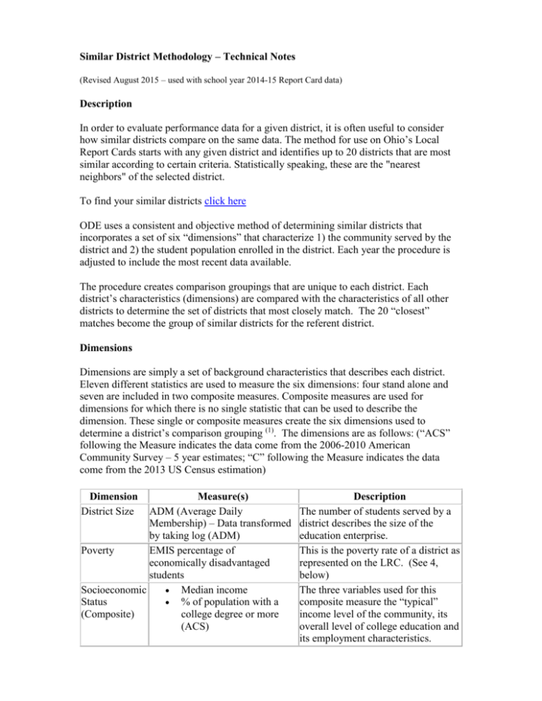
Similar District Methodology – Technical Notes
(Revised August 2015 – used with school year 2014-15 Report Card data)
Description
In order to evaluate performance data for a given district, it is often useful to consider
how similar districts compare on the same data. The method for use on Ohio’s Local
Report Cards starts with any given district and identifies up to 20 districts that are most
similar according to certain criteria. Statistically speaking, these are the "nearest
neighbors" of the selected district.
To find your similar districts click here
ODE uses a consistent and objective method of determining similar districts that
incorporates a set of six “dimensions” that characterize 1) the community served by the
district and 2) the student population enrolled in the district. Each year the procedure is
adjusted to include the most recent data available.
The procedure creates comparison groupings that are unique to each district. Each
district’s characteristics (dimensions) are compared with the characteristics of all other
districts to determine the set of districts that most closely match. The 20 “closest”
matches become the group of similar districts for the referent district.
Dimensions
Dimensions are simply a set of background characteristics that describes each district.
Eleven different statistics are used to measure the six dimensions: four stand alone and
seven are included in two composite measures. Composite measures are used for
dimensions for which there is no single statistic that can be used to describe the
dimension. These single or composite measures create the six dimensions used to
determine a district’s comparison grouping (1). The dimensions are as follows: (“ACS”
following the Measure indicates the data come from the 2006-2010 American
Community Survey – 5 year estimates; “C” following the Measure indicates the data
come from the 2013 US Census estimation)
Dimension
District Size
Measure(s)
ADM (Average Daily
Membership) – Data transformed
by taking log (ADM)
Poverty
EMIS percentage of
economically disadvantaged
students
Socioeconomic
 Median income
Status
 % of population with a
(Composite)
college degree or more
(ACS)
Description
The number of students served by a
district describes the size of the
education enterprise.
This is the poverty rate of a district as
represented on the LRC. (See 4,
below)
The three variables used for this
composite measure the “typical”
income level of the community, its
overall level of college education and
its employment characteristics.
Rural/Urban
Continuum
(Composite)

% of population in
administrative/professional
occupations (ACS)




Population density
% of agricultural property
Population (C)
Incorporation of a city
larger than 40,000 (C)
This composite uses four variables to
create a continuous measure that
distinguishes school districts that
have urban characteristics from those
that have more rural characteristics.
% of students enrolled reported as
African-American, Hispanic,
This is a measure of the racial/ethnic
Native-American, or Multiracial.
Race/Ethnicity
diversity of the student population in
Data transformed by taking log
the district.
(base 10). If % is less than 1%,
log is set at “0”.
NonThis is a measure of community's
Agricultural
Per-pupil amount of commercial,
ability to generate revenue for
and Nonindustrial, mining, tangible, and
schools-separate from its residential
Residential
public utility property
(or agricultural) tax base.
Tax Capacity
How the data are analyzed
Each district is compared to 609 other districts by performing a comparison across all
dimensions (2). The result is a “distance” between each pair of districts. The smaller the
“distance,” the more similar the two districts are. For each district, the 20 “closest”
districts are selected as its group of similar districts. In some cases, the distance between
a district and its closest neighbors is very large. In these cases, there can be fewer than 20
“similar districts” reflecting the unique features of the referent district.
Limitations
Developing similar district comparison groupings is a process that enables individual
districts to conduct meaningful comparative analysis. Despite the benefits to this
approach, there are limitations to the use of the methodology. The concerns that impact
these limitations are outlined below.
1. The method does not include a geographical dimension. Many districts tend to
compare themselves with surrounding districts. The similar district method does not
necessarily include geographically close districts in the given district's performance
comparison grouping because neighboring districts might not truly be the most
similar districts in the state. On the other hand, expenditure patterns (expenditures per
pupil, salary information, etc.) tend to reflect regional conditions. Thus, a better way
to compare financial data is to select districts that are geographically close.
2. The method deliberately selects the “nearest” 20 districts as the standard for
comparison. But some districts are more “unique” than others. In some cases
(typically very large cities), “distances” to other districts are so large that a cut-off
point needs to be established in the distance metric, which limits the comparison
group to fewer than 20. An arbitrary minimum number of similar districts for any
district is five.
It is also true that some districts tend to look like many other districts, so the cutoff of
20 similar districts captures those districts that are extremely similar according to the
chosen dimensions. In this case, districts can closely resemble many other districts
beyond the cutoff of 20. Small, rural districts often fall into this category.
3. Generating unique comparison groupings can produce seemingly counter-intuitive
results if inter-grouping comparisons are made. Stated another way, laying out
several similar district groupings side by side and making comparisons across several
groupings may be tempting but is not appropriate given the method. The following
example illustrates why this is so.
Tables 1, 2, and 3 (below) contain FY2015 comparison groupings for Southwestern
City, Lakewood City, and Reynoldsburg City. Note the following:



Lakewood and Reynoldsburg both appear in Southwestern’s comparison
groupings.
Southwestern appears in Lakewood’s comparison grouping (but not in
Reynoldburg’s).
Lakewood and Reynoldsburg do not appear in each other's comparison groupings.
This occurs because each district's comparison grouping is unique to itself and
contains only the 20 “nearest” districts (maximum). Comparisons across similar
groupings are not appropriate because the similar grouping method establishes like
districts for a given district ONLY. Southwestern is statistically similar to both
Lakewood and Reynoldsburg. While Lakewood’s list includes Southwestern but not
Reynoldsburg, Reynoldsburg’s comparison grouping includes neither Southwestern
nor Lakewood.
4. Starting with the data for school year 2007-08, the percent poverty measure is the rate
reported through EMIS using the economic disadvantagement flag. In prior years this
measure was based on poverty counts reported by the Ohio Department of Job and
Family Services pursuant to ORC 3317.10. These are two different (although highly
correlated) measures and caution should be taken in comparing the two.
Questions
For questions or comments, contact:
Matthew Cohen, Chief Research Officer
Office of Policy and Research
Ohio Department of Education
25 S. Front Street, 4th Floor
Columbus, Ohio 43215
(614) 752-8729
Matt.Cohen@education.ohio.gov
(1) Tests for relationships between data elements were conducted with each variable prior
to the analysis of dimensions. Data representing each dimension were normalized
prior to the analysis, with means equal to zero and standard deviations of 1. This
process standardized the metric used for comparative purposes so that each district
can be fairly compared with any other district.
(2) The formula for each district-to-district comparison is as follows. Where A, B, C, D,
E, and F represent dimension values; i represents the district of interest; and j
represents the district being compared to that district, then the distance “O” between
two districts is calculated as:
O = ((Ai-Aj)2 + (Bi-Bj)2 + (Ci-Cj)2 + (Di-Dj)2 + (Ei-Ej)2+ (Fi-Fj)2) 1/2
Table 1 - Southwestern FY 2015 Comparison Grouping
1
2
3
4
5
6
7
8
9
10
11
12
13
14
15
16
17
18
19
20
Southwestern City CSD
Northwest Local
Washington Local
Fairfield City
Hamilton City
Parma City
Elyria City
Newark City
Huber Heights City
Willoughby-Eastlake City
Plain Local
Kettering City
Groveport-Madison Local
Findlay City
Euclid City
Canton City
Berea City
Westerville City
Lakewood City
Fairborn City
Reynoldsburg
Franklin
Hamilton
Lucas
Butler
Butler
Cuyahoga
Lorain
Licking
Montgomery
Lake
Stark
Montgomery
Franklin
Hancock
Cuyahoga
Stark
Cuyahoga
Franklin
Cuyahoga
Greene
Franklin
Table 2 - Lakewood FY 2015 Comparison Grouping
1
2
3
4
5
6
7
8
9
10
11
12
13
14
15
16
17
18
19
20
Lakewood City SD
Cuyahoga Falls City
Parma City
Plain City
Kettering City
Northwest Local
Fairfield City
Westerville City
Huber Heights City
Willoughby-Eastlake City
Findlay City
Washington Local
Fairborn City
Berea City
Cleveland Hts-University Hts City
Newark City
West Clermont Local
South Western City
Mentor Exempted
Euclid City
Oak Hills Local
Cuyahoga
Summit
Cuyahoga
Stark
Montgomery
Hamilton
Butler
Franklin
Montgomery
Lake
Hancock
Lucas
Greene
Cuyahoga
Cuyahoga
Licking
Clermont
Franklin
Lake
Cuyahoga
Hamilton
Table 3 - Reynoldsburg FY 2015 Comparison Grouping
1
2
3
4
5
6
7
8
9
10
11
12
13
14
15
16
17
18
19
20
Reynoldsburg City
Huber Heights City
Northwest Local
Plain Local
Northmont City
Fairborn City
Springfield Local
West Carrollton City
Winton Woods City
Austintown Local
Findlay City
Licking Heights Local
Fairfield City
Xenia Community City
South Euclid-Lyndhurst City
Delaware City
Mad River Local
Kent City
Garfield Heights City
Groveport-Madison Local
Canal Winchester Local
Franklin
Montgomery
Hamilton
Stark
Montgomery
Greene
Lucas
Montgomery
Hamilton
Mahoning
Hancock
Licking
Butler
Greene
Cuyahoga
Delaware
Montgomery
Portage
Cuyahoga
Franklin
Franklin