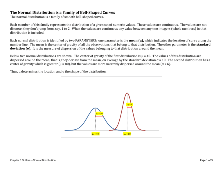
The Normal Distribution is a Family of Bell-Shaped Curves
The normal distribution is a family of smooth bell-shaped curves.
Each member of this family represents the distribution of a given set of numeric values. These values are continuous. The values are not
discrete; they don’t jump from, say, 1 to 2. When the values are continuous any value between any two integers (whole numbers) in that
distribution is included.
Each normal distribution is identified by two PARAMETERS: one parameter is the mean (µ), which indicates the location of curve along the
number line. The mean is the center of gravity of all the observations that belong to that distribution. The other parameter is the standard
deviation (σ). It is the measure of dispersion of the values belonging to that distribution around the mean.
Below two normal distributions are shown. The center of gravity of the first distribution is µ = 40. The values of this distribution are
dispersed around the mean, that is, they deviate from the mean, on average by the standard deviation σ = 10. The second distribution has a
center of gravity which is greater (µ = 80), but the values are more narrowly dispersed around the mean (σ = 6).
Thus, µ determines the location and σ the shape of the distribution.
σ₂ = 6
σ₁ = 10
μ₁ = 40
Chapter 3 Outline—Normal Distribution
μ₂ = 80
Page 1 of 9
How to Determine Probability of 𝒙 Values in a Normal Distribution
A continuous random variable can take on infinite number of values within an interval of numbers. Since the normal distribution is the
distribution of a continuous random variable, the probability of any specific value is zero. Therefore, probability is defined only for an
interval of values of a normal random variable, and is the area under the normal curve belonging to that interval.
Example
A normally distributed random variable X has a mean of μ = 60 and a standard deviation of σ = 8.
What is the probability that 𝑥 is less than (less than or equal to) 52?
What is the probability that x is less than (less than or equal to) 70?
P(𝑥 < 52) = P(𝑥 ≤ 52) = ________
P(𝑥 < 70) = P(𝑥 ≤ 70) = ________
52
60
x
60
Transform 𝑥 to 𝑧 (standard normal)
𝑥 − μ 52 − 60
𝑧=
=
= −1.00
σ
8
𝑧=
70
x
𝑥 − μ 70 − 60
=
= 1.25
σ
8
P(𝑧 < 1.25) = 0.8944
P(𝑧 < −1.00) = 0.1587
0.8944
0.1587
-1.00
Chapter 3 Outline—Normal Distribution
0
z
0
1.25
z
Page 2 of 9
μ = 60
σ=8
“Closed” intervals
P(52 < 𝑥 < 68) = ______
60
52
68
P(44 < 𝑥 < 76) = ______
x
𝑥 − μ 68 − 60
𝑧=
=
= 1.00
σ
8
𝑧=
52 − 60
= −1.00
8
0
76
x
76 − 60
= 2.00
8
𝑧=
84 − 60
= 3.00
8
𝑧=
44 − 60
= −2.00
8
𝑧=
36 − 60
= −3.00
8
0.6544
1.00
P(z < 1.00) = 0.8413
P(z < -1.00) = 0.1587
P(-1.00 < z < 1.00) = 0.6826
Chapter 3 Outline—Normal Distribution
z
60
36
𝑧=
0.6826
-1.00
60
44
P(36 < 𝑥 < 84) = ______
-2.00
0
P(z < 2.00) = 0.9772
P(z < -2.00) = 0.0228
P(-2.00 < z < 2.00) = 0.9544
84
x
0.9974
2.00
z
-3.00
0
3.00 z
P(z < 3.00) = 0.9987
P(z < -3.00) = 0.0013
P(-3.00 < z < 3.00) = 0.9974
Page 3 of 9
Example
Vehicle speed on a freeway is normally distributed with a mean of 77 mph (μ = 77) and standard deviation of 8 mph (σ = 8).
What proportion of vehicles drive below 65
mph?
P(x < 65) = ______
65
𝑧=
77
What proportion of vehicles drive above 90
mph?
P(x > 90) = _______
x
65 − 77
= −1.50
8
77
𝑧=
0
𝑃(𝑧 < −1.50) = 0.0668
Chapter 3 Outline—Normal Distribution
z
90
What proportion of vehicles drive between
65 and 89 mph?
P(65 < x < 89) = ______
x
90 − 77
= 1.63
8
65
𝑧=
0
P(z > 1.63) = 1 – P(z < 1.63)
P(z > 1.63) = 1 – 0.9484 = 0.0516
z
77
65 − 77
= −1.50
8
89
𝑧=
x
89 − 77
= 1.50
8
0
z
P(z < 1.50) = 0.9332
P(z < −1.50) = 0.0668
P(-1.50 < z < 1.50) = 0.8664
Page 4 of 9
μ = 77
σ=8
What proportion of vehicles drive within ±10 mph from the mean.
What proportion drive within ±1.8 standard deviations from the
mean speed?
NOTE: ±1.8 standard deviations from the mean simply represent the z-scores. The
z-score, by definition, is the deviation from the mean expressed in units of σ.
P(μ − 10 < 𝑥 < μ + 10) = P(67 < 𝑥 < 87)
P(μ − 1.8σ < 𝑥 < μ + 1.8σ) = P(62.6 < 𝑥 < 91.4)
77
z = (67 – 77) ∕ 8 = -1.25
x
77
z = (87 – 77) ∕ 8 = 1.25
z = (62.6 – 77) ∕ 8 = -1.80
0
P(𝑧 < 1.25) = 0.8944
P(𝑧 < −1.25) = 0.1056
P(−1.25 < 𝑧 < 1.25) = 0.7888
Chapter 3 Outline—Normal Distribution
x
z = (91.4 – 77) ∕ 8 = 1.80
z
0
z
P(z < 1.80) = 0.9641
P(z < -1.80) = 0.0359
P(-1.80 < z < 1.80) = 0.9282
Page 5 of 9
Changing Directions
In the examples below, the probability is given and you are asked to find the interval of x values that is associated with that probability.
Vehicle speed on a freeway is normally distributed with a mean of 77 mph (μ = 77) and standard deviation of 8 mph (σ = 8).
Below what speed 30% (or 0.30 proportion) of vehicles drive?
Above what speed 20% (or 0.20 proportion) of vehicles drive?
x = ? 77
x
Using the z-table, first find the z score that corresponds to an area
(probability) that is closest to 0.30:
z = -0.52
-0.52 0
𝑧=
𝑥−μ
σ
𝒙 = μ + 𝒛𝛔
77 x = ?
x
Using the z-table, first find the z score that corresponds to an area
(probability) that is closest to 0.80:
z = 0.84
z
0 0.84
z
𝑥 = μ + 𝑧σ
𝑥 = 77 + 0.84(8) = 83.7 mph
𝑥 = 77 + (−0.52)(8) = 72.8 mph
Chapter 3 Outline—Normal Distribution
Page 6 of 9
Given, μ = 77 and σ = 8
The speed above which 10% (or 0.10
proportion) of vehicles drive is:
P(x > ____) = 0.10
77
x
The speed above which 5% (or 0.05
proportion) of vehicles drive is:
P(x > ____) = 0.05
x
The z-score that bounds a tail are of 0.10 is
𝒛𝟎.𝟏𝟎 = 𝟏. 𝟐𝟖
0
1.28
x
77
The speed above which 2.5% (or 0.025
proportion) of vehicles drive is:
P(x > ____) = 0.025
x
The z-score that bounds a tail are of 0.05 is
𝒛𝟎.𝟎𝟓 = 𝟏. 𝟔𝟒
z
0
1.65
77
x
The z-score that bounds a tail are of 0.025 is
𝒛𝟎.𝟎𝟐𝟓 = 𝟏. 𝟗𝟔
z
0
𝑥 = μ + 𝑧σ
𝑥 = μ + 𝑧σ
𝑥 = μ + 𝑧σ
𝑥 = 77 + 1.28(8) = 87.2 mph
𝑥 = 77 + 1.64(8) = 90.1 mph
𝑥 = 77 + 1.96(8) = 92.7 mph
P(𝑥 > 87.2) = 0.10
P(𝑥 > 90.1) = 0.05
P(𝑥 > 92.7) = 0.025
Chapter 3 Outline—Normal Distribution
x
1.96
z
Page 7 of 9
Given, μ = 77 and σ = 8
The middle speed interval which contains
80% (or 0.80) of all vehicles is: ____ to ____
P(____ < 𝑥 < ____) = 0.80
0
P(____ < 𝑥 < ____) = 0.90
x
77
-1.28
The speed interval which contains 90% (or
0.90) of all vehicles is: ____ to ____
1.28
z
0
P(____ < 𝑥 < ____) = 0.95
x
77
-1.64
The speed interval which contains 95% (or
0.95) of all vehicles is: ____ to ____
1.64
z
-1.96
0
𝑥𝐿 = 77 + (−1.28)(8) = 66.8
𝑥𝐿 = 77 + (−1.64)(8) = 63.9
𝑥𝐿 = 77 + (−1.96)(8) = 61.3
𝑥𝑈 = 77 + (1.28)(8) = 87.2
𝑥𝑈 = 77 + (1.64)(8) = 90.1
𝑥𝑈 = 77 + (1.96)(8) = 92.7
𝑃(66.8 < 𝑥 < 87.2) = 0.80
𝑃(63.9 < 𝑥 < 90.1) = 0.90
𝑃(61.3 < 𝑥 < 92.7) = 0.95
Chapter 3 Outline—Normal Distribution
x
77
1.96
z
Page 8 of 9
On a different highway 5% of vehicles drive above 75 miles per hour.
The standard deviation of vehicle speed is σ = 5. The mean vehicle
speed is μ = _____.
Yet, on another highway 2.5% of vehicle drive above 62 mph. The
mean speed is 54 mph. The standard deviation of vehicle speed is σ
= ____.
𝑥 = μ + 𝑧σ
μ = 𝑥– 𝑧σ
z0.05 = 1.64
σ=5
µ = 75 – 1.64(5) = 66.8 mph
𝑧=
𝑥−μ
σ
σ=
𝑥−μ
𝑧
z0.025 = 1.96
σ=
Chapter 3 Outline—Normal Distribution
62 − 54
= 4.1 mph
1.96
Page 9 of 9