2101
Bivariate Linear Regression
Bivariate Linear Regression analysis involves finding the best fitting straight line to describe a
set of bivariate data. It is based upon the linear model, Y a bX e . That is, every Y score is
made up of two components: a + bX, which is the linear "effect" of X upon Y, the value of Y given X if
X and Y were perfectly correlated in a linear fashion, and e, which stands for error. Error is simply
the difference between the actual value of Y and that value we would predict from the best fitting
straight line. That is, e Y Yˆ
Sources of Error
There are three basic sources that contribute to the error term, e.
Error in the measurement of X and or Y or in the manipulation of X (experimental research).
The influence upon Y of variables other than X (extraneous variables), including variables that
interact with X.
Any nonlinear influence of X upon Y.
The Regression Line
The best fitting straight line, or regression line, is Yˆ a bX , or, in z-score units, Zˆ y rZ x
If r2 is less than one (a nonperfect correlation), then predicted Zy "regresses" towards the
mean relative to Zx.
The criterion used to find the best fitting straight line is the least squares criterion. That is,
2
we find a and b such that Y Yˆ is as small as possible. This is the same criterion used to
define the mean of a univariate distribution. The regression line is an extension of the concept of a
mean into two-dimensional space.
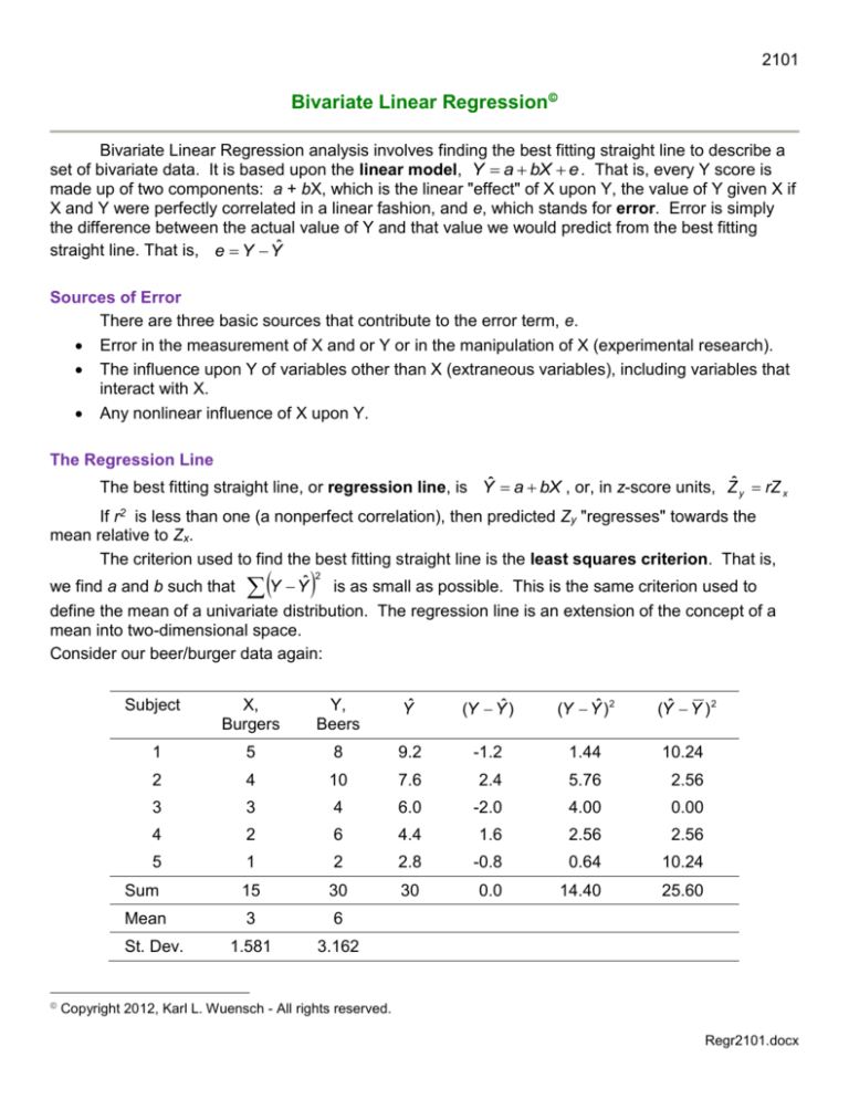
Consider our beer/burger data again:
Subject
X,
Burgers
Y,
Beers
Yˆ
(Y Yˆ )
(Y Yˆ ) 2
(Yˆ Y ) 2
1
5
8
9.2
-1.2
1.44
10.24
2
4
10
7.6
2.4
5.76
2.56
3
3
4
6.0
-2.0
4.00
0.00
4
2
6
4.4
1.6
2.56
2.56
5
1
2
2.8
-0.8
0.64
10.24
Sum
15
30
30
0.0
14.40
25.60
Mean
3
6
1.581
3.162
St. Dev.
Copyright 2012, Karl L. Wuensch - All rights reserved.
Regr2101.docx
SSY 4(3.162) 2 40
The b is the slope, the amount that predicted Y changes for each one unit increase in X. We
sy
SSCP COVxy
shall compute the slope by: b
. For our beer-burger data,
r
SS x
sx
s x2
3.162
b .8
1 .6
1.581
Please note that if sy = sx, as would be the case if we changed all scores on Y and X to zscores, then r = b. This provides a very useful interpretation of r. Pearson r is the number of
standard deviations that predicted Y changes for each one standard deviation change in X. That is,
on the average, and in sd units, how much does Y change per sd change in X.
We compute the intercept, a, the predicted value of Y when X = 0, with: a Y bX . For our
data, that is 6 – 1.6(3) = 1.2
Variance Due to Error or Due to Regression
One may wish to estimate the error term in the linear model. The error sum of squares is:
2
SSE Y Yˆ SS 1 r 2 . SSE is the quantity we minimized when solving for a and b. To
y
convert SSE into an estimate of the population error variance or residual variance (the average
SSE
squared deviation between Y and predicted Y in the population) one computes: MSE
. MSE
n2
stands for mean square error. This mean is also known as the estimated residual variance. It
represents the variance in the Y scores that is not due to Y’s linear association with X. That is, it is
the variance in Y due to extraneous variables, nonlinear effects, and slop in the measurement and/or
manipulation of X and Y. If we did not know X or if r = 0, our best (least squares) prediction for Y
would be the mean of Y, regardless of the value of X, and SSE Y Y SSy . Since SSE
would then = SSy, all of the variance in Y would be error variance. If r is nonzero we can do better
than just always predicting Yˆ Y , and SSE will be less than SSy. If we wish to get our estimate of
average error of prediction back to our original units rather than squared units, we compute the
n 1
standard error of estimate, s y yˆ MSE s y 1 r 2
. For our beer-burger data, where the
n2
14.4
4.8 , and the standard
total SS for Y was 40, SSE (1 r 2 )(SSy ) (1 .64)( 40) 14.4 , MSE
3
error of estimate is 4.8 2.191.
SSE represents the SS in Y not due to the linear association between X and Y. SSregr, the
regression sum of squares, represents the SS in Y that is due to that linear association.
SSregr Yˆ Y
2
2
SSy SSE r 2 SSy . For our beer-burger data, that is 40 - 14.4 = 25.6.
The mean square regression, MSregr
SSregr
, where p is the number of predictor variables
p
(X’s). Since in bivariate regression we have only one X variable, p = 1 and MSregr = SSregr.
SS regr
The coefficient of determination, r 2
. That is, r2 represents the proportion of the
SS y
variance in Y that is accounted for by the linear association between X and Y. The coefficient of
2
alienation, 1 r 2
SSerror
is the proportion of the variance in Y that is not accounted for by that linear
SSy
association.
Look back at the first table, the one with the data. Notice that I included the predicted scores
2
2
and the residuals. Notice that Y Yˆ 0 , Y Yˆ SS , and Yˆ Y SS
.
error
regression
Testing Hypotheses
The most common hypothesis tested in simple regression analysis is the hypothesis that in the
population the slope for predicting Y from X is zero. That is, using a linear regression to predict Y
from X is no better than always predicting Y = the mean on Y. Student's t may be employed,
t
MSregr
, df n 2 . This will yield exactly the same t and p obtained were you to test the
MSE
hypothesis that population r = 0, but the assumptions are less restrictive.
One may also test the null hypothesis of a zero slope using an F-statistic (Analysis of
MSregr
Variance). F
. It is evaluated on p degrees of freedom in the numerator and (n - p - 1) df in
MSE
the denominator, where p = the number of predictor (independent) variables (1 for bivariate
regression). Note that this is another case where a one-tailed test is appropriately used to test
nondirectional hypotheses. Also note that F = t2. The one-tailed p obtained for our ANOVA (see
table below) is exactly the same as the two-tailed p we earlier obtained employing t to test the null
hypothesis that is zero in the population. The square root of the F below is equal to the value of
that t computed earlier.
The results of the test of the hypothesis of a zero slope may be summarized in an ANOVA
(analysis of variance) source table. For our beer-burger data, here is such a table:
SS
df
MS
F
p
Regression
25.6
1
25.6
5.33
.104
Error
14.4
3
4.8
Total
40.0
4
10.0
Source
The MStotal is nothing more than the sample variance of the dependent variable Y. It is usually
omitted from the table.
Constructing a Confidence Interval for R2
First you need to decide whether your predictor variable is random or fixed. Then you need to
read my document Putting Confidence Intervals on R2 or R. For our current example the predictor
variable is random.
Effect Size
The r or r2 statistic is a standardized effect size statistic. Cohen’s guidelines for effect sizes
are:
3
ρ
.1
.3
.5
Effect size
Small
Medium
Large
ρ2
.01
.09
.25
Presenting the Results
Our summary statement might read something like this: “A .05 criterion of statistical
significance was employed for all tests. The linear regression between my friends’ burger
consumption and their beer consumption fell short of statistical significance, r = .8, beers =
1.2 + 1.6 burgers, F(1, 3) = 5.33, p = .10. A 95% confidence interval for ρ runs from -.28 to .99.
The most likely explanation of the nonsignificant result is that it represents a Type II error.
Given our small sample size (N = 5), power was only 17% even for a large effect (ρ = .5).
More Data, More Power
Suppose that we wisely decided to repeat the experiment, but with a larger sample size, 10
friends. Suppose the following source table was obtained:
SS
df
MS
F
p
Regression
25.6
1
25.6
5.33
.05
Error
38.4
8
4.8
Total
64.0
9
7.1
Source
Note that with the same F (but more error df), our effect is now significant. The r2 is going to
equal SSregression divided by SStotal, that is, 25.6/64.0 = .4.
If we used t to test the null hypothesis, t
.632 8
1 .40
2.31, and the exact two-tailed p for that t
on 8 df is .05.
Our summary statement might read something like this: “A .05 criterion of statistical
significance was employed for all tests. An a priori power analysis indicated that our sample
size (N = 10) would yield power of only 32% even for a large effect (ρ = .5). Despite this low
power, our analysis yielded a statistically significant result. Among my friends, beer
consumption increased significantly with burger consumption, r = .632, beers = 1.2 + 1.6
burgers, F(1, 8) = 5.33, p = .05.” A 95% confidence interval for ρ runs from .005 to .90.
Suppose that we were going to test directional hypotheses, testing the alternative hypothesis
that slope in the population is greater than 0. For t, our one-tailed p would be half of the two-tailed p,
that is, p = .025. With F, our (half-tailed) p would be half of the one-tailed p, that is, p = .025. One
way to understand this “half-tailed” p is this: If the null hypothesis were true (the slope is zero in the
population), what would be your chances of getting a sample slope whose absolute value was as
large (or larger) than that you obtained? The answer is our one-tailed p, .05. Now, what would be
your chances of guessing the direction (positive or negative) of the obtained slope (before the data
are collected) if you really were just guessing? The answer there is .5. Now, were the null
hypothesis true, what would be the probability of your correctly guessing the direction of the slope
and getting a slope whose absolute value is that far from zero? Using the multiplication rule of
4
probability under the assumption of independence, your chances would be (.5)(.05) = .025, our “halftailed” probability.
No assumptions are necessary to use r, a, b, s y yˆ , etc. as descriptive statistics or to use MSE
as an unbiased estimate of population error variance.
Placing Confidence Limits on Predicted Values of Y
1. If we are using the regression line to predict the mean value of Y for all subjects who have
some particular score on X, Yˆ X , it might be advisable to report an interval within which we are
relatively confident that the true (population) value of mean Y given X falls. How confident is
relatively confident? Very often the criterion is 95%, (1 - ). To compute such a confidence interval
1 XX
we use: CI Yˆ t s y yˆ
n
SS x
2
.
2. If we wish to estimate an individual value of Y given X we need to widen the confidence
interval to include the variance of individual values of Y given X about the mean value of Y given X ,
1 XX
using this formula: CI Yˆ t s y yˆ 1
n
SS x
2
.
3. In both cases, the value of t is obtained from a table where df = n - 2 and (1 - cc)/2 = the
upper tail p used to locate critical t. Recall that cc is the confidence coefficient, the degree of
confidence desired.
4. Constructing confidence intervals requires the same assumptions as hypothesis testing the
slope.
5. The confidence intervals about the regression line will be bowed [see them], with that for
predicting individual values wider than that for predicting average values.
Testing Other Hypotheses
One may test the null hypothesis that the slope for predicting Y from X is the same in one
population as it is in another. For example, is the slope of the line relating blood cholesterol level to
blood pressure the same in women as it is in men? We shall not cover such a test in this course.
Should you need to conduct such a test, consult an advanced statistics text. Please do note that this
test is not equivalent to a test of the null hypothesis that two correlation coefficients are equal.
The Y.X relationships in different populations may differ from one another in terms of slope,
intercept, and/or scatter about the regression line (error, 1 - r2). [See relevant plots] There are
methods (see Kleinbaum & Kupper, Applied Regression Analysis and Other Multivariable Methods,
Duxbury, 1978, Chapter 8) to test all three of these across two or more groups.
Suppose that for predicting blood pressure from blood cholesterol the slope were exactly the
same for men and for women. The intercepts need not be the same (men might have higher average
blood pressure than do women at all levels of cholesterol) and the r's may differ, for example, the
effect of extraneous variables might be greater among men than among women, producing more
scatter about the regression line for men, lowering r2 for men. Alternatively, the r's may be identical
but the slopes different. For example, suppose the scatter about the regression line was identical for
men and women but that blood pressure increased more per unit increase in cholesterol for men than
for women.
5
Distinction Between Correlation and Regression
Correlation and regression are very closely related topics. Technically, if the X variable (often
called the “independent variable, even in nonexperimental research) is fixed, that is, if it includes all
of the values of X to which the researcher wants to generalize the results, and the probability
distribution of the values of X matches that in the population of interest, then the analysis is a
regression analysis. If both the X and the Y variable (often called the “dependent” variable, even in
nonexperimental research) are random, free to vary (were the research repeated, different values
and sample probability distributions of X and Y would be obtained), then the analysis is a correlation
analysis. For example, suppose I decide to study the correlation between dose of alcohol (X) and
reaction time. If I arbitrarily decide to use as values of X doses of 0, 1, 2, and 3 ounces of 190 proof
grain alcohol and restrict X to those values, and have the equal numbers of subjects at each level of
X, then I’ve fixed X and do a regression analysis. If I allow X to vary “randomly,” for example, I recruit
subjects from a local bar, measure their blood alcohol (X), and then test their reaction time, then a
correlation analysis is appropriate.
In actual practice, when one is using linear models to develop a way to predict Y given X, the
typical behavioral researcher is likely to say she is doing regression analysis. If she is using linear
models to measure the degree of association between X and Y, she says she is doing correlation
analysis.
Assumptions
No assumptions are necessary to use r, a, b, s y yˆ , etc. as descriptive statistics or to use MSE
as an unbiased estimate of population error variance. If, however, you use t or F to test hypotheses
or construct confidence intervals, then there are assumptions.
In a regression analysis we consider the X variable to be fixed rather than random.
Accordingly, the assumptions are different than those used in correlation analysis.
We have already discussed the assumptions associated with hypothesis testing and
confidence interval estimation when considering both X and Y as random variables (a correlation
analysis) – homoscedasticity and bivariate normality.
When we consider the predictor variable(s) to be fixed (a regression analysis), there are no
assumptions about the predictor (X) variable(s). We do assume homogeneity of variance
(homoscedasticity) in the distributions of Y given X, that is, variance in Y is not a function of X, is
constant across X. We also assume that the conditional distribution of Y is normal at every value of
X. These assumptions can be restated in terms of the error term: The distribution of the error term
(the residuals) is normal at every value of X and constant in variance across values of X.
More on Assumptions in Correlation and Regression
Copyright 2012, Karl L. Wuensch - All rights reserved.
6
