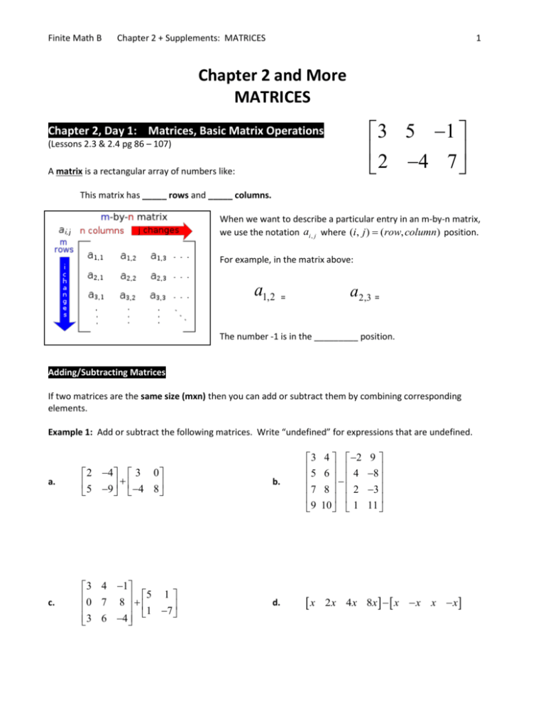
Finite Math B
Chapter 2 + Supplements: MATRICES
1
Chapter 2 and More
MATRICES
3 5 1 
 2 4 7 


Chapter 2, Day 1: Matrices, Basic Matrix Operations
(Lessons 2.3 & 2.4 pg 86 – 107)
A matrix is a rectangular array of numbers like:
This matrix has _____ rows and _____ columns.
When we want to describe a particular entry in an m-by-n matrix,
we use the notation ai , j where (i, j )  ( row, column) position.
For example, in the matrix above:
a1,2
a2,3 =
=
The number -1 is in the _________ position.
Adding/Subtracting Matrices
If two matrices are the same size (mxn) then you can add or subtract them by combining corresponding
elements.
Example 1: Add or subtract the following matrices. Write “undefined” for expressions that are undefined.
a.
 2 4   3 0 
 5 9    4 8 

 

b.
3
5

7

9
c.
3 4 1
 0 7 8   5 1 

 1 7 

3 6 4 
d.
x
4   2
6   4

8  2
 
10  1
9
8
3

11 
2 x 4 x 8x    x  x x  x 
Finite Math B
Chapter 2 + Supplements: MATRICES
Multiplication by a Scalar Factor:
2
Multiply each entry in the matrix by the factor
 b c   ab ac 
a


 d e   ad ae 
Example 2: Simplify. Write undefined for any expression that may be undefined.
a.
 x 
3  8 y 
 7 z 
2 3x 
x

b. 2 x 4 y 2 y
3 

 1 0 2 x 
Multiplying Matrices
Let A be an m x n matrix
Let B be an n x k matrix
To find the product:
Multiply each element in the row of A by the
corresponding element in the column of B, then add
these products.
The product matrix AB is an m x k matrix.
SAMPLE:
Find the product AB
 2 3 1
A

4 2 2 
1 
B  8 
6
A is 2 x 3
B is 3 x 1
AB will be 2 x 1
Step 1: Multiply the elements of the first row of A and
the corresponding elements in the column of B.
Example 3:
Find the product
 2
2 4 6   
 1 3 0   3

  4
 
2(1) + 3(8) + -1(6) = 20
Step 2: Multiply the elements of the second row of A
and the corresponding elements in the column of B.
4(1) + 2(8) + 2(6) = 32
Step 3: Write your solution as a 2 x 1 matrix.
 20 
 32 
 
Finite Math B
Chapter 2 + Supplements: MATRICES
3
Example 4: Find the product. Write “undefined for expressions that are undefined.
 2 1  3 
a) 
 
 5 8   2 
 0 2
 2 2 1 

b) 
  1 4
3
0
1

  0 2


 2 1  1 0 4 
c) 


 3 6  5 2 0 
 1 1 2  2 3
 3 2 1   3 2
d)



 4 5 2  4 5 
Finite Math B
Chapter 2 + Supplements: MATRICES
4
Example 4 (continued): Find the product. Write “undefined for expressions that are undefined.
e)
 2 5 3  1 2 3
7 4 6  3 2 1 



 3
 2 2 4 6 1
f)

 
1 
Finite Math B
Chapter 2 + Supplements: MATRICES
5
Chapter 2, Day 2: Determinants and Cramer’s Rule
A determinant is a special number associated with a square matrix. The determinant has several useful
applications in algebra and other advanced mathematics courses.
Notation:
a b 
c d 


Matrix Notation (square brackets)
2x2
Determinant Notation (straight brackets)
a b
2x2
c d
(This notation represents “find the determinant of the matrix”)
Also: det(A) or detA represents “the determinant of matrix A”
2x2 Matrices
The determinant of a 2 x 2 matrix is found as follows:
Example 1: Find the determinant of each 2 x 2 matrix
3 4 

5 6 
a) 
 1 3 

 6 7 
b) 
Example 2: Find each determinant.
a)
2
3
5 10
b)
2 7
3 5
c)
x x
7 8
a b

3x3 d e

 g h
c
f 
i 
a b
3x3 d e
g h
c
f
i
Finite Math B
Chapter 2 + Supplements: MATRICES
6
3x3 Matrices
The determinant of a 3x3 matrix is found as
follows:
This is easier to find using a little trick called
“The Rule of Sarrus”:
1. Copy the first two columns next to column 3.
2. Multiply the three “southeast”
(downward)diagonals. Find the sum.
3. Multiply the three “northeast” (upward)
diagonals. Find the sum.
4. Determinant = (SE sum) – (NE sum)
bottom – top
Example 3: Find the determinant of each matrix.
a)
1 3 5 
2 1 3


 4 5 2 
b)
1
Watch out!
Example 4: Evaluate
2
3
1 2 3
3 2 1
 2 3 1
 4 2 3 


 2 2 1 
Finite Math B
Chapter 2 + Supplements: MATRICES
7
Cramer’s Rule
4 x  5 y  17

3 x  2 y  7
Matrices can be used to solve systems of linear equations.
solution:
Remember that a system of equations is two or more equations.
A solution is any ordered pair (or higher) that satisfies the equation.
 3, 1
A system of equations has three potential solution types:
Cramer’s Rule is a method of solving systems of linear equations using matrices instead of the methods you
learned in Algebra (Substitution/Elimination/Graphing).
Example 1: Solve using Cramer’s Rule
4 x  5 y  17

3x  2 y  7
Step 1: Write the system of equations as a
coefficient matrix and an answer matrix.
Step 2: Find the determinant of the
coefficient matrix. This is called “D”.
Step 5:
x
Dx
Dy
, y
D
D
Step 3: Replace the “x” column of
the coefficient matrix with
answer column. Find determinant. This is called Dx.
Step 4: Replace “y” column of
the coefficient matrix with
answer column. Find determinant. This is called Dy.
Step 6: Check your answer!!!
Finite Math B
Chapter 2 + Supplements: MATRICES
8
Example 2: Solve using Cramer’s Rule
a)
c)
b)
Finite Math B
Chapter 2 + Supplements: MATRICES
Example 2 (Continued) : Solve using Cramer’s Rule
d)
e)
9
Finite Math B
Chapter 2 + Supplements: MATRICES
10
Chapter 2, Day 3: Using Technology
Working with Matrices in the TI 83/TI83plus/TI84 Graphing Calculator
TI-83 Matrix Menu
About the Matrix (MATRX) menu:
MATRX
2nd
x-1

NAMES – used to paste the name
of a matrix into the home screen
or into a program.

MATH – contains all the
operations that can be done with
a matrix.

EDIT – where you set the size of
the matrix and enter the
elements.
Note: Some TI 83 models do not require you to “shift” to access the matrix menu.
BASIC OPERATIONS
Use the graphing calculator to perform the following operations:
1.
2.
 2 4   3 0 
 5 9    4 8 

 

 2 4   3 0 
 5 9   4 8 



3.
 2 4   1
 5 9   4 

 
4.
 2 4 
5

 5 9 
5.
 3
 2 2 4 6 1

 
1 
6.
 2 5 3  1 2 3
7 4 6  3 2 1 



Finite Math B
Chapter 2 + Supplements: MATRICES
11
DETERMINANTS
In the matrix menu, use the EDIT screen to enter your matrix.
Use 2nd (MODE) to quit to the main screen.
In the matrix menu, use the MATH screen to paste det( into your home screen and the NAMES screen to paste
the name of the matrix. Close ) and hit enter
Use the graphing calculator to find the determinant of each of the following matrices.
2
7.
3
5 10
8.
1 3 5 
2 1 3


 4 5 2 
1
9.
CRAMER’S RULE
Solve using Cramer’s Rule: Be sure to show the values of D, Dx, Dy, and Dz (if applicable)
10.
11.
2
3
1 2 3
3 2 1
Finite Math B
Chapter 2 + Supplements: MATRICES
12
Chapter 2, Day 4: Row Operations and The Gauss-Jordan Method
Row Operations
We will be using “Row Operations” to manipulate matrices to help us solve systems and canvas.
What you are allowed to do:
1. INTERCHANGE TWO ROWS
Example: Interchange R1 and R2
 2 1 1 2 


1 3 2 1 
1 1 1 2 
2. MULTIPLY THE ELEMENTS OF A ROW BY A NONZERO REAL NUMBER
Example: 3  R1  R1
 2 1 1 2 


1 3 2 1 
1 1 1 2 
3. ADD A NONZERO MULTIPLE OF THE ELEMENTS OF ONE ROW TO THE CORRESPONDING ELEMENTS OF A
NONZERO MULTIPLE OF SOME OTHER ROW.
Example: 2  R3  R1  R1
 2 1 1 2 


1 3 2 1 
1 1 1 2 
Gauss-Jordan Method
Strategy:
1. Write the system of equations as an augmented matrix
2. Use Row Operations to transform the matrix into a matrix with whole numbers on the main diagonal, but 0’s
elsewhere.
3. Use Row Operations to transform the matrix into an “identity” matrix.
(1’s on diagonal, 0’s elsewhere)
3. Final solution = numbers in the “answer” column of the matrix.
Example:
Meaning:
1 0 3

1
0 1 5 
Example:
Meaning:
1 0 0 4 


0 1 0 2 
0 0 1 3 
Finite Math B
Chapter 2 + Supplements: MATRICES
13
Example : Use the Gauss-Jordan Method to solve each system of equations
Make it happen:
Your Goal:
1 0 0 # 
1 0 # 


 0 1 #  or  0 1 0 # 


 0 0 1 # 
Using legal row operations:
# # #
0 # #


# # # #
0 # # #


 0 # # # 
a)
2 x  4 y  2

3 x  5 y  0
b)
3x  4 y  1

5 x  2 y  19
# 0 #
0 # #


1 0 # 
0 1 #


# 0 # #
0 # # #


 0 0 # # 
# 0 0 #
0 # 0 #


 0 0 # # 
1 0 0 # 
0 1 0 #


 0 0 1 # 
Finite Math B
Chapter 2 + Supplements: MATRICES
Example (Continued): Use the Gauss-Jordan Method to solve each system of equations
c)
x  2 y  2

3 x  6 y  5
d)
x yz 3
2x  3y  7z  0
x  3 y  2 z  17
14
Finite Math B
Chapter 2 + Supplements: MATRICES
Example (Continued): Use the Gauss-Jordan Method to solve each system of equations
2x  5 y  4z  8
e)
f)
2x  2z  4
x  2 y  z  2
x  y  5 z  6
3 x  3 y  z  10
x  3y  2z  5
15
Finite Math B
Chapter 2 + Supplements: MATRICES
16
Working with Matrices in the TI 83/TI83plus/TI84 Graphing Calculator
Reduced Row Echelon Form (Gauss Jordan Result)
Using the TI83 Graphing Calculator to solve a system of equations
5 x  2 y  z  5

3x  3 y  3z  9
x  2 y  4z  6

INSTRUCTIONS
1. In the matrix menu, use the EDIT screen to enter the
augmented matrix that represents your system.
2. Quit to the home screen.
3. Go to MATRX and MATH.
Scroll down and hit ENTER to select B: rref(
4. Go to MATRX and NAMES. Hit ENTER to paste [A] to your
home screen. Close the parenthesis.
5. Press ENTER and read the solution from the matrix.
You Try: Use the Graphing Calc to solve:
x  y  5 z  6
3 x  3 y  z  10
x  3y  2z  5
Finite Math B
Chapter 2 + Supplements: MATRICES
17
Chapter 2, Day 5: Modeling and Solving Using Matrices
Set up an augmented matrix to represent the problem. Use Cramer’s Rule, Gauss Jordan, or a
graphing calculator to solve the system of equations and answer the given question.
Example 1: (ex. 6 pg 78-80)
A convenience store sells 23 sodas one summer afternoon in 12-oz, 16-oz, and 20-oz cups (small, medium, and
large). The total volume of soda sold was 376 oz. Suppose the prices for a small, medium, and large soda are
$1, $1.25, and $1.40, respectively, and that the total sales were $28.45. How many of each size did the store
sell?
Example 2: (exercise #45 pg 83)
A knitting shop orders yarn from three suppliers in Toronto, Montreal, and Ottawa. One month the shop
ordered a total of 100 units of yard from these suppliers. The delivery costs were $80, $50, and $65 per unit for
the orders from Toronto, Montreal, and Ottawa, respectively, with a total delivery cost of $5990. The shop
ordered the same amount from Toronto and Ottawa. How many units were ordered from each supplier?
Finite Math B
Chapter 2 + Supplements: MATRICES
18
Example 3: (exercise #46 pg 83)
An electronics company produces three models of stereo speakers, models A, B, and C, and can deliver them by
truck, van, or station wagon. A truck holds 2 boxes of model A, 2 of model B, and 3 of model C. A van holds 3
boxes of model A, 4 boxes of model B, and 2 boxes of model C. A station wagon holds 3 boxes of model A, 5
boxes of model B, and 1 box of model C.
a) If 25 boxes of model A, 33 boxes of model B, and 22 boxes of model C are to be delivered, how many vehicles
of each type should be used so that all operate at full capacity?