ASEN 2002
Aeronautics Experiment: Aerodynamics of Cylinders and Wings
Assigned 26 OCT, Due 18 NOV
OBJECTIVES
• Introduction Bernoulli’s equation for incompressible flow.
•
Introduction to external, incompressible flow around simple geometric shapes.
•
Introduction to flow measurements and wind tunnel testing.
•
Introduction to two-dimensional flow and airfoil theory.
BACKGROUND
Bernoulli’s Equation and Airspeed Measurements
The incompressible Bernoulli equation can be derived from the momentum conservation law (Newton’s 2 nd
law) or as a special statement of conservation of energy,
(1.1)
In English, this equation states that the sum of the static pressure (potential energy) and dynamic pressure
(kinetic energy) is equal to the constant total pressure (total energy). This equation is valid on a streamline when we can ignore forces that dissipate energy, i.e. viscous forces (friction).
Pressure is one of the few flow quantities that is easily measured and Bernoulli’s equation gives us a relatively simple means of indirectly measuring flow speed by measuring pressure. We can write Eq. (1.1) as an expression for the speed in terms of a difference between the total and static pressures,
(1.2)
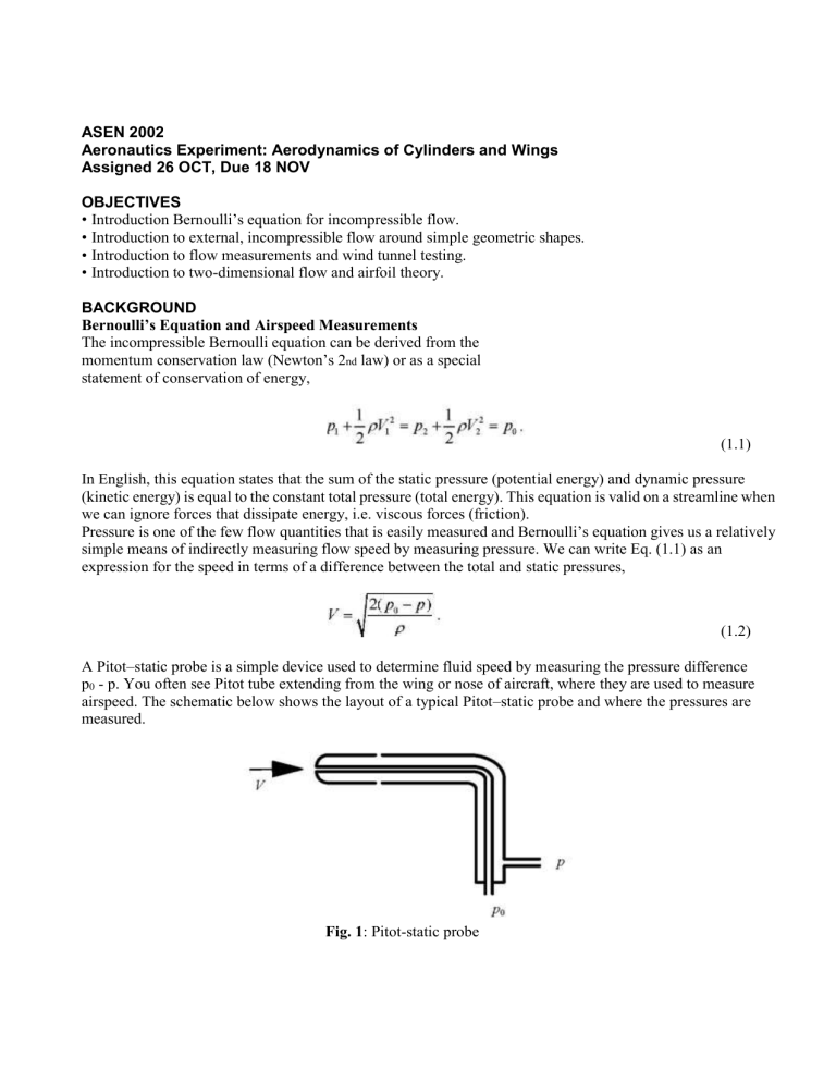
A Pitot–static probe is a simple device used to determine fluid speed by measuring the pressure difference p
0
- p. You often see Pitot tube extending from the wing or nose of aircraft, where they are used to measure airspeed. The schematic below shows the layout of a typical Pitot–static probe and where the pressures are measured.
Fig. 1 : Pitot-static probe

It is common engineering practice to write quantities in terms of dimensionless coefficients. This enables results from measurements obtained under different conditions to be correlated. This is how, for instance, measurements made on a scale model in a wind tunnel are scaled to full size aircraft. As an example of an important dimensionless quantity we define the coefficient of pressure,
(1.3) where the subscript ∞ denotes the free-stream value far upstream of an object in the undisturbed flow and q ∞ is the dynamic pressure. The coefficient of pressure contains information for how pressure varies on the surface of an immersed object. Using Bernoulli’s equation, we can directly relate the speed on the surface of the object to the coefficient of pressure,
(1.4)
Finally, the Pitot–tube speed relation can be written such that it gives the speed of the undisturbed flow approaching an object, so Eq. (1.2) becomes,
Conversely, it gives the speed of an object moving into a quiescent fluid.
(1.5)
The Low-Speed Wind Tunnel
Figure 4 shows a schematic of the wind tunnel setup. The objective of this experiment is to measure the two-dimensional pressure distribution on the surface of circular cylinder and separately, to measure the pressure distribution on the surface of an airfoil, and then to integrate this pressure distribution over the surface to determine the lift and drag (pressure component only for drag). We will use a circular cylinder and a small wing section, each fitted with “pressure taps” spaced over a two-dimensional cross-section of each model. Pressure taps are small holes drilled in the wing surface which are connected to a pressure transducer via a network of small tubes. Each tap samples the pressure at that point. Thus we will sample the pressure distribution at 12 points on the cylinder and 20 points on the airfoil. While this gives us a fairly crude picture of the pressure distribution, for the cylinder it provides enough resolution to compare the actual flow to the ideal flow, and for the airfoil it provides enough data to estimate the lift coefficient and the pressure drag.

Fig. 2: Wind tunnel Schematic
Flow Around a Circular Cylinder: Limitations of Hydrodynamic Theory
Hydrodynamics is the study of “perfect” fluids, i.e., fluids that are incompressible (constant density) and inviscid (no viscosity, thus frictionless). Hydrodynamic theory matured following the publication of Isaac
Newton’s Philosophiæ Naturalis Principia Mathematica (1687), usually referred to as the Principia , which laid the groundwork for advanced dynamical analysis. The theory is purely mathematical in nature, thus sometimes does not agree with observation. It is however, a very elegant theory that, under the right circumstances, can accurately describe certain features of a fluid flow. One of the more famous shortcomings of hydrodynamic theory is referred to as d’Alembert’s paradox
(Anderson p. 359). This “paradox” states that an object immersed in a perfect fluid has no drag. That is, according to the theory, an object moving through a fluid has no tendency to slow down. The pressure cylinder experiment will provide an opportunity to explore what physical features of a real flow cannot be captured by hydrodynamic theory, thus resulting in a failure of the theory.
Fig. 3: Ideal frictionless flow around a circular cylinder

Figure 3 shows the streamlines (lines which particles of fluid move along) around a cross section of a circular cylinder immersed in a perfect fluid. Below the cylinder cross section is a diagram that shows the variation of the coefficient of pressure on the cylinder surface, as predicted from hydrodynamic theory. The theory predicts where θ is the azimuthal angle measured as shown.
(2.1)
Note that a negative value of C p
indicates a local pressure that is below the free-stream value p ∞ , and a positive value indicates a local pressure above p ∞ .
How Wings Produce Lift
A wing is a three–dimensional shape that, when immersed in an appropriate flow, will produce a usable force from a pressure imbalance. As shown in Fig. 4, an airfoil is a two–dimensional cross section of a wing, sliced in the direction of the incident flow. The airfoil displays the aerodynamic shape used to produce a pressure imbalance. The net force of the pressure imbalance (in a real fluid, frictional forces are also present), summed over the wing, is resolved into lift and drag. By definition, lift is the net force component perpendicular to the flow and drag is the net force component parallel to the flow. This experiment focuses on lift.
Fig. 4: Wing features
The design of a wing generally begins with the airfoil. The airfoil schematic in Fig. 5 shows some of the associated nomenclature. Once the airfoil is designed to produce a certain pressure imbalance and associated lift, a wing is constructed by projecting the airfoil into the third dimension, i.e., the span-wise dimension. Other things may be done to tailor the performance of the wing such as using different airfoil sections over the span, or introducing twist by slightly rotating sections as one moves outward in span. Additionally, airfoils are usually designed to keep the flow attached over as much of the surface as possible to prevent the type of flow you observed over the circular cylinder. There is a tremendous literature describing the large number of airfoils developed primarily for aeronautical applications over the past 100 years. Many of these airfoils were developed from the classical thin airfoil theory, the focus of our current analysis.

Fig. 5: Airfoil nomenclature
Before proceeding, let us define the nondimensional parameter called the coefficient of lift,
(3.1) where L is the lift, q ∞ is the dynamic pressure, and S is the reference area. Remember, dimensionless coefficients such as C
L
enable us to scale experimental results from sub–scale models to full–scale vehicles.
Another thing to note is by writing Eq. (3.1) in the form
(3.2) we can examine the operational procedures of a fixed-wing airplane from takeoff to landing. For incompressible flow, and a fixed-wing geometry, Eq. (3.2) shows that for a fixed coefficient of lift C
L
, the lift is directly proportional to the square of the speed. This means that the faster the wing moves through the air, the more lift is generated. That is why an airplane has to pick up speed down the runway before it is able to takeoff. In order to takeoff, the wings (the entire vehicle) must produce more lift than the total gross weight of the aircraft (gross weight is the absolute total weight, i.e., including passengers, luggage, fuel, etc.). When the airplane is cruising at a constant altitude, the lift only has to balance, not exceed, the weight.
Thin airfoil theory begins with hydrodynamic theory and can accurately predict the lift (but not the drag—d’Alambert’s paradox) of a “thin” airfoil, at relatively low angle of attack. In the airfoil schematic above, notice that the shape is not symmetrical, in fact the average shape is curved. The curvature in the airfoil shape is called camber . Note that if the upper and lower surfaces are identical in shape, the mean camber line and the chord line coincide and the airfoil is symmetrical . A cambered airfoil will produce lift when the angle of attack
(specifically the geometric angle of attack) is zero.

Everyone who has driven, or ridden in a car has probably held a hand out an open window as if it were a wing.
You certainly noticed that when you incline your hand it is either forced up or down, depending on the angle of attack. To lift your hand, you raise the “leading edge” upward. This is also done with winged bodies such as airplanes. As mentioned previously, when you see an airplane takeoff, it first builds up speed along the runway, then the pilot rotates the vehicle to increase the angle of attack α of the wing. From experience we know that increasing the α of our hand increases the amount of lift, to a certain point (at some point, your hand tends to fly more backwards than upwards). Thin airfoil theory gives us a very simple relation between lift and the angle of attack. In terms of the coefficient of lift C l
, this relation is
(3.3) where α
0
is the angle for zero lift (which is related to the airfoil camber). Earlier we used the symbol C
L
to denote the lift coefficient for an entire wing. When working with airfoils, as we are now, we use the symbol
C l
= l/(q
∞ c)where l is the lift per unit span and c is the airfoil chord.
Just how realistic is thin airfoil theory? Would you expect to see a deviation from this theory for the case of a real airfoil? That is what you will determine from the experiment. So, we shift back to the question of how lift is produced. We mentioned earlier that lift results from an imbalance of pressure forces on the upper and lower surface of the wing. With the wind tunnel and an appropriately instrumented airfoil model, we can measure the distribution of pressure on the upper and lower surface. Knowing the distribution of pressure on the upper and lower surface, we can integrate (sum) all the contributions to determine the net force perpendicular to the air flow, i.e., the lift. By repeating this exercise for several angles of attack, we can then construct a plot to see how the pressure distributions and the lift vary with α. Any ideas of how these distributions may appear for the wing stalls ? What about a non-symmetric wing at zero angle of attack?
The schematic in Fig. 6 shows a typical pressure distribution on an airfoil that is producing lift. Here the pressure is cast in terms of the non-dimensional pressure coefficient. Note that the plot is inverted and shows negative values of C p
in the upper half-plane and positive values in the lower half-plane. From the definition of
C p
we see that a negative C p
value means the pressure is lower than the free-stream pressure, p ∞ and positive values correspond to pressures higher than p ∞ . So, when a wing produces lift, the upper surface generally has a net negative C p
distribution (a net suction), while the lower surface generally has, but not always, a net positive
C p
distribution. The relatively lower pressure on the upper surface and the relatively higher pressure on the lower surface work together to produce lift.

Fig. 6 Pressure distribution on the upper and lower surface of an airfoil.
Force Integration Procedure
As discussed above, we must integrate the pressure distribution in order to calculate the lift and pressure drag.
Since we sample the pressure at a discrete number of points, we must resort to a numerical integration. This procedure described below Fig. 7 that shows the airfoil section along with the coordinate systems to be used.
Lift and drag ( L and D ) are defined relative to the oncoming flow direction. The normal and axial forces ( n and a ) are referenced with respect to the airfoil. It is easiest to perform the force integrations in the airfoil coordinate system (thereby determining n and a ) and then transfer these forces to the free-stream coordinate system (giving the desired L and D ).
Let the pressure tap locations be denoted as ( x i
, y i
) and the corresponding pressure be p i
where i = 1, 2, ..., n . In order to perform the force integrations we will break the airfoil surface into linear elements, each of which span two consecutive pressure taps. Such an element, spanning taps i and i + 1, is shown in Fig. 7. We shall assume that the pressure is constant over each element and equal to the average of the pressures at the two end points
(where the taps are located). According to the sketch, the normal force over the i th
segment is
(3.4)
The sketch shows that cosθ = Δx i
/ Δs i
, so that Eq. (3.4) can be simplified to give
(3.5)

Fig. 7 Surface element for force integration.
A similar development shows that the axial force is given by
Summing over all elements gives the total forces
(3.6)
(3.7)
(3.8)
Note that Δx i
= x i+1
- x i
and Δy i
= y i+1
- y i
. It is convenient to rewrite the force expressions in non-dimensional form. We accomplish this by adding and subtracting the free-stream pressure ( p ∞ ) from the right hand side and then dividing both sides by the quantity ½ρ
∞ v
∞
2 c , where c is the airfoil chord. The result for the normal force is

The definition of the pressure coefficient is evident above and the last term vanishes since the summation is taken over a closed contour (the airfoil surface). Making these simplifications, and performing the analogous operations on the expression for the axial force gives
(3.10)
(3.11)
Notice that these expressions are nothing more than trapezoidal rule approximations to the following two contour integrals which give the exact normal and axial force coefficients
(3.12)
(3.13)
In order to get the lift and drag, it is necessary to transfer the normal and axial force coefficients to the free-stream coordinate system. With reference to Fig. 7 it is easy to show that
(3.14)
(3.15)
If the angle of attack is small we see that the lift is dominated by the normal force and the drag is dominated by the axial force.
By breaking the contour integrals shown in Eqs. (3.12) and (3.13) into two parts, one for the upper surface and one for the lower surface, it is possible to write the equivalent forms
(3.16)
(3.17) where the subscripts u and l refer to the upper and lower surfaces respectively and dy/dx is the surface slope.
These equations can be found in Chapter 5 of Anderson. Although these forms are not the most convenient for our data analysis, they are useful in understanding how lift is produced. In particular, if the angle of attack is small, then C l
~C n
. We see that the above expression for C l
~C n
represents the cross-hatched area under the curves in the schematic of Fig. 6. In other words, Eq. (3.16) says the sectional lift coefficient is equal to the difference between the pressure coefficient evaluated on the lower surface and upper surface, integrated along the chord line. Look again at the schematic that shows the pressure distribution for a wing producing lift. The integral in Eq. (3.16) represents the cross hatched area between the C pu
and C pl
curves. Since C pu
is negative, note that the negative sign in Eq. (3.16) causes the C pu
contribution to be positive, so that the two portions of the integral are both positive.

Experimental Procedure
Cylinder
1.
Calculate the air density within the ITL from the pressure and temperature displayed on the LabView screen. Use these values to compute the Reynolds number Re.
2.
Examine the pitot probe. Make sure it is level.
3.
Align the cylinder such that pressure port #1 is aligned normal to the free stream.
4.
Click the “zero airspeed” and “zero pressure” buttons to zero the pressure transducers.
5.
Watch the pressure traces on the LabView screen for several seconds and record the minimum and maximum pressure readings prior to starting the wind tunnel. This will give a measure of the uncertainty in the pressure measurements.
6.
Set the airspeed to 25 m/s in the appropriate box and hit enter. Monitor the airspeed readout as the fan stabilizes.
7.
Using the pressure tap selector button, step through all 12 pressure taps (0° to 180° in 15° increments).
After changing to each new setting, wait a few seconds for the pressure readings to stabilize and then click the “save values to file” button.
8.
Repeat steps 6 and 7 for speed of 20 m/s and 30 m/s.
Wing
1.
Calculate the air density within the ITL from the pressure and temperature displayed on the LabView screen. Use these values to compute the Reynolds number Re.
2.
Examine the pitot probe. Make sure it is level.
3.
Set the wing to the desired angle of attack. To do this, proceed as follows: a.
Using an Allen wrench, loosen the four set screws that lock the turntable in place (the screws are located on the exterior of the wind tunnel, under the test section) b.
Rotate the turntable to the desired angle of attack as measured by the the scale on the floor of the test section. To rotate the turntable, press down on it slightly as you apply rotational forces with your fingers. DO NOT USE THE WING AS LEVER TO ROTATE THE TURNTABLE
AS THIS MIGHT DAMAGE THE WING OR THE PRESSURE TUBES . c.
Tighten the set screws to lock the turntable in place.
4.
Enter the angle of attack setting in the appropriate box on the LabView screen.
5.
Click the “zero airspeed” and “zero pressure” buttons to zero the pressure transducers.
6.
Watch the pressure traces on the LabView screen for several seconds and record the minimum and maximum pressure readings prior to starting the wind tunnel. This will give a measure of the uncertainty in the pressure measurements.
7.
Enter the desired airspeed in the appropriate box and hit enter. Monitor the airspeed readout as the fan stabilizes.
8.
Using the pressure tap selector button, step through all 19 pressure taps. After changing to each new setting, wait a few seconds for the pressure readings to stabilize and then click the “save values to file” button.

Data Analysis
You will share your data with all other lab groups in order to form a composite data base. Perform the following for each set of your pressure measurements.
1.
Convert the pressures to non-dimensional pressure coefficients.
2.
Write a MatLab procedure to integrate the pressure distribution around the airfoil, thereby obtaining the normal and axial force coefficients. The preferred numerical integration formulas are given in Eqs.
(3.10) and (3.11). In order to apply these equations directly, the last element (element 20) needs to join element 1 at the leading edge, thereby forming a closed contour. This feature can be accomplished easily by including data for a virtual pressure tap 21, which is identical to tap 1. Operationally, this can be achieved by copying the data for tap 1, placing it at the end of the file, and relabeling it as tap 21. A computer program can then step through each element, summing up the terms given in Eqs. (3.10) and
(3.11).
3.
Convert the normal and axial force coefficients to lift and drag coefficients without making any small angle approximations.
4.
Upload your C l
and C d
values to the course repository via CULearn.
5.
Download the composite C l
and C d
file, also from CULearn.
Data Presentation
1.
Plot the composite collection of pressure coefficients C p
vs. azimuthal angle θ on the cylinder surface for the three Reynolds number cases, compared to the ideal case (compare means multiple curves on a single plot; see Fig. 5.70 in Anderson)
2.
Plot the pressure coefficient C p
vs. x / c for each case that you measured. Plot the data in the customary fashion with negative C p
values plotted above the x axis (see Fig. 5.13 in Anderson).
3.
Plot the composite collection of lift coefficients C l
as a function of the angle of attack α. Use distinct symbols (with no connecting lines) for the data at 15 m/s and 30 m/s. Include the thin airfoil result as a solid line. You will need to determine the zero lift angle of attack to do this.
4.
Make a similar plot for the drag coefficient. The thin airfoil prediction for the drag is that it is zero for all angles of attack. Include this for reference.
Topics for Discussion
1.
Compare and describe the observed flow about the circular cylinder with that predicted for an ideal frictionless fluid.
2.
Where is the stagnation point on the cylinder, how does it compare to the Pitot-static probe reading?
3.
Can you determine where boundary-layer separation occurs?
4.
Explain why there is a differential between the pressures on the upper and lower surfaces when the airfoil is positioned at an angle of attack. How does this pressure difference translate into lift and drag?
5.
Explain the observed variations in lift and drag with changes in angle of attack. How is stall identified?
6.
Compare the observed lift and drag variations with the thin airfoil theory. Comment on any systematic departures from the theory.
7.
Explain why or why not the non-dimensional data from different tunnel speeds should collapse.
Comment on any systematic variations in the force coefficients with Reynolds number (tunnel speed).
8.
Explain why or why not you are able to measure frictional drag in this experiment.