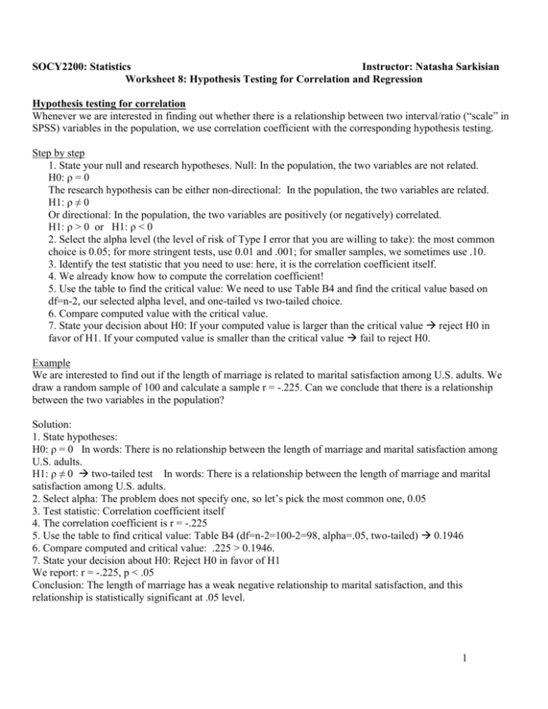
SOCY2200: Statistics
Instructor: Natasha Sarkisian
Worksheet 8: Hypothesis Testing for Correlation and Regression
Hypothesis testing for correlation
Whenever we are interested in finding out whether there is a relationship between two interval/ratio (“scale” in
SPSS) variables in the population, we use correlation coefficient with the corresponding hypothesis testing.
Step by step
1. State your null and research hypotheses. Null: In the population, the two variables are not related.
H0: ρ = 0
The research hypothesis can be either non-directional: In the population, the two variables are related.
H1: ρ ≠ 0
Or directional: In the population, the two variables are positively (or negatively) correlated.
H1: ρ > 0 or H1: ρ < 0
2. Select the alpha level (the level of risk of Type I error that you are willing to take): the most common
choice is 0.05; for more stringent tests, use 0.01 and .001; for smaller samples, we sometimes use .10.
3. Identify the test statistic that you need to use: here, it is the correlation coefficient itself.
4. We already know how to compute the correlation coefficient!
5. Use the table to find the critical value: We need to use Table B4 and find the critical value based on
df=n-2, our selected alpha level, and one-tailed vs two-tailed choice.
6. Compare computed value with the critical value.
7. State your decision about H0: If your computed value is larger than the critical value  reject H0 in
favor of H1. If your computed value is smaller than the critical value  fail to reject H0.
Example
We are interested to find out if the length of marriage is related to marital satisfaction among U.S. adults. We
draw a random sample of 100 and calculate a sample r = -.225. Can we conclude that there is a relationship
between the two variables in the population?
Solution:
1. State hypotheses:
H0: ρ = 0 In words: There is no relationship between the length of marriage and marital satisfaction among
U.S. adults.
H1: ρ ≠ 0  two-tailed test In words: There is a relationship between the length of marriage and marital
satisfaction among U.S. adults.
2. Select alpha: The problem does not specify one, so let’s pick the most common one, 0.05
3. Test statistic: Correlation coefficient itself
4. The correlation coefficient is r = -.225
5. Use the table to find critical value: Table B4 (df=n-2=100-2=98, alpha=.05, two-tailed)  0.1946
6. Compare computed and critical value: .225 > 0.1946.
7. State your decision about H0: Reject H0 in favor of H1
We report: r = -.225, p < .05
Conclusion: The length of marriage has a weak negative relationship to marital satisfaction, and this
relationship is statistically significant at .05 level.
1
Hypothesis Testing for Regression
In regression, we use hypothesis tests to determine if our independent variable X has an effect on the dependent
variable Y in the population. In a bivariate regression model, we obtain two coefficients: constant a and
intercept b. In principle, we could test hypotheses for both of them, but usually, we are not interested whether
our constant, a, is different from 0 or not. So the more important test is for the slope b. If we find that the slope
is significantly different from zero, we conclude that there is in fact a linear relationship between the
independent and dependent variables in the population.
Step by Step
1. State your null and research hypotheses. Null: In the population, the independent variable has no
effect on the dependent variable.
H0: β = 0
The research hypothesis can be either non-directional: In the population, the independent variable has
an effect on the dependent variable. H1: β ≠ 0
Or directional: In the population, an increase in the independent variable is associated with an increase
(or decrease) in the dependent variable.
H1: β > 0 or H1: β < 0
2. Select the alpha level (the level of risk of Type I error that you are willing to take): the most common
choice is 0.05; for more stringent tests, use 0.01 and .001; for smaller samples, we sometimes use .10.
3. Identify the test statistic that you need to use: Student’s t
4. Formula: t = b/SEb
SEb is the standard error of our regression slope b; if you manually calculated b, you would have to
calculate SEb as
Here, y is values of our y, y’ is predicted values of y based on the regression equation, x is values of x,
is the mean of x, and n is the sample size. We won’t calculate it by hand in this class though.
5. Use the table to find the critical value: We need to use Table B2 and find the critical value based on
df=n-2, our selected alpha level, and one-tailed vs two-tailed choice.
6. Compare computed value with the critical value.
7. State your decision about H0: If your computed value is larger than the critical value  reject H0 in
favor of H1. If your computed value is smaller than the critical value  fail to reject H0.
Example
We expect that among employed Americans, those who spend more time commuting by car have higher levels
of stress as a result. We use a nationally representative sample of 75 employed individuals and regress stress
on time spent commuting by car. We end up obtaining slope b = 0.247, with a standard error of .133. Can we
conclude that commuting time increases stress among Americans?
Solution:
1. State hypotheses:
H0: β = 0 In words: The commuting time has no effect on stress among Americans.
H1: β > 0 In words: The commuting time increases stress among Americans.
2. Select alpha: 0.05
2
3. Test statistic: Student’s t
4. t = b/sb = .247/.133 = 1.86
5. Use the table to find critical value: Table B2 (df=n-2 = 75-2=73, alpha = .05, one-tailed)  1.666
6. Compare computed & critical value: 1.86 > 1.666
7. State your decision: We reject H0 in favor of H1.
Conclusion: The time spent commuting by car is associated with increased levels of stress among employed
Americans, and this relationship is statistically significant at .05 level.
Exercises
1. We are interested to find out if one’s income is related to life satisfaction. We draw a random sample
of 50 and calculate a sample r = .455. Can we conclude that there is a relationship between the two
variables in the population?
2. We expect that higher levels of job autonomy lead to higher levels of employee satisfaction. We use
a nationally representative sample of 65 employed individuals and regress employee satisfaction on
job autonomy. We end up obtaining slope b = 0.372, with a standard error of .199. Can we conclude
that job autonomy increases employee satisfaction?
3
3. Use variables AGEKDBRN and TVHOURS to evaluate whether, in the U.S. population, there is a
relationship between the age when one has their first child and the number of hours watching TV. [Note:
State hypotheses, use SPSS, and state your conclusions.]
4.
Use variables AGE and TVHOURS to evaluate whether, as Americans get older, they watch more
hours of TV per day. [Note: State hypotheses, use SPSS, and state your conclusions.]
4