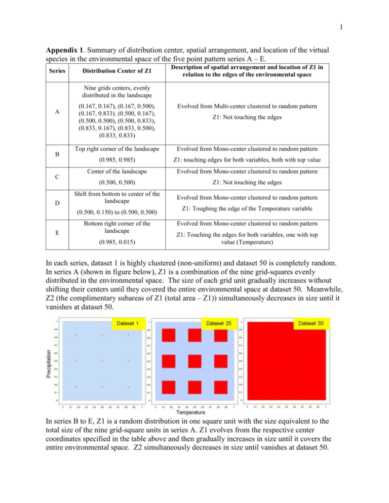
1
Appendix 1. Summary of distribution center, spatial arrangement, and location of the virtual
species in the environmental space of the five point pattern series A – E.
Series
Distribution Center of Z1
Description of spatial arrangement and location of Z1 in
relation to the edges of the environmental space
Nine grids centers, evenly
distributed in the landscape
A
B
C
D
(0.167, 0.167), (0.167, 0.500),
(0.167, 0.833). (0.500, 0.167),
(0.500, 0.500), (0.500, 0.833),
(0.833, 0.167), (0.833, 0.500),
(0.833, 0.833)
Evolved from Multi-center clustered to random pattern
Top right corner of the landscape
Evolved from Mono-center clustered to random pattern
(0.985, 0.985)
Z1: touching edges for both variables, both with top value
Center of the landscape
Evolved from Mono-center clustered to random pattern
(0.500, 0.500)
Z1: Not touching the edges
Shift from bottom to center of the
landscape
Evolved from Mono-center clustered to random pattern
(0.500, 0.150) to (0.500, 0.500)
E
Bottom right corner of the
landscape
(0.985, 0.015)
Z1: Not touching the edges
Z1: Toughing the edge of the Temperature variable
Evolved from Mono-center clustered to random pattern
Z1: Touching the edges for both variables, one with top
value (Temperature)
In each series, dataset 1 is highly clustered (non-uniform) and dataset 50 is completely random.
In series A (shown in figure below), Z1 is a combination of the nine grid-squares evenly
distributed in the environmental space. The size of each grid unit gradually increases without
shifting their centers until they covered the entire environmental space at dataset 50. Meanwhile,
Z2 (the complimentary subareas of Z1 (total area – Z1)) simultaneously decreases in size until it
vanishes at dataset 50.
In series B to E, Z1 is a random distribution in one square unit with the size equivalent to the
total size of the nine grid-square units in series A. Z1 evolves from the respective center
coordinates specified in the table above and then gradually increases in size until it covers the
entire environmental space. Z2 simultaneously decreases in size until vanishes at dataset 50.
2
Appendix 2. Visualization of basic types of point patterns. Uniform pattern describes the
spatial pattern in which the density of points in any subarea of the interested region is equal if the
size and shape being the same. Conversely, non-uniform pattern describes the pattern with the
density of points varies between one subarea and the other. Quantitatively, a regular point
pattern (a) means the distance between each point and their paired points remains the same for
one or more specified directions (in this case vertical and horizontal) within the focused area;
while a random point pattern (b) means the probability of containing a point in one subarea is the
same as any other subarea of the same size and shape, regardless of the location of these
subareas. A gradient pattern means (c) the probability of locating one individual point varies
inversely with distance to the points have already been located from single-clustered center;
while a clustered pattern (d) means probability of locating one individual point varies inversely
with distance to the points have already been located, but allowed to have multi-clustered
centers.
a
b
c
d
3
Appendix 3. Binned calibration method. Red line corresponds to the perfect calibration of the
model, where the plotted points fall on the 1:1 line. The coefficient of the regression line (black)
represents the overall calibration of each run from the individual datasets (1 to 50) of each series
4
Appendix 4. Point patterns of species occurrence data in the extracted environmental space
(from the native range) for Prosopis farcta (A) and Imperata cylindrica (B), represented by the
component scores of the dimension reduction results of PCA. Red dots represent the occurrence
data locations reflected in the environmental space. Boundaries of the environmental space
correspond to their environmental space within the native ranges. The extents of the
environmental space reflect the relative size of the native ranges for these two species
2.862