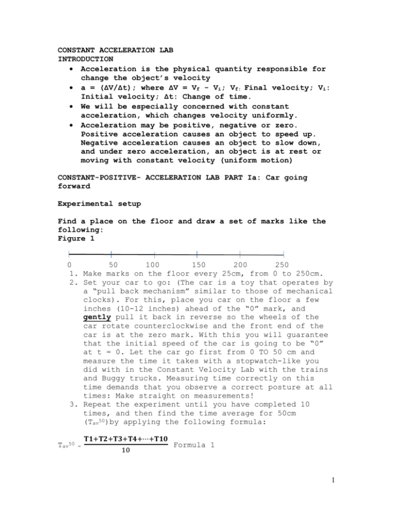
CONSTANT ACCELERATION LAB
INTRODUCTION
 Acceleration is the physical quantity responsible for
change the object’s velocity
 a = (ΔV/Δt); where ΔV = Vf - Vi; Vf: Final velocity; Vi:
Initial velocity; Δt: Change of time.
 We will be especially concerned with constant
acceleration, which changes velocity uniformly.
 Acceleration may be positive, negative or zero.
Positive acceleration causes an object to speed up.
Negative acceleration causes an object to slow down,
and under zero acceleration, an object is at rest or
moving with constant velocity (uniform motion)
CONSTANT-POSITIVE- ACCELERATION LAB PART Ia: Car going
forward
Experimental setup
Find a place on the floor and draw a set of marks like the
following:
Figure 1
0
50
100
150
200
250
1. Make marks on the floor every 25cm, from 0 to 250cm.
2. Set your car to go: (The car is a toy that operates by
a “pull back mechanism” similar to those of mechanical
clocks). For this, place you car on the floor a few
inches (10-12 inches) ahead of the “0” mark, and
gently pull it back in reverse so the wheels of the
car rotate counterclockwise and the front end of the
car is at the zero mark. With this you will guarantee
that the initial speed of the car is going to be “0”
at t = 0. Let the car go first from 0 TO 50 cm and
measure the time it takes with a stopwatch-like you
did with in the Constant Velocity Lab with the trains
and Buggy trucks. Measuring time correctly on this
time demands that you observe a correct posture at all
times: Make straight on measurements!
3. Repeat the experiment until you have completed 10
times, and then find the time average for 50cm
(Tav50)by applying the following formula:
Tav50
𝐓𝟏+𝐓𝟐+𝐓𝟑+𝐓𝟒+⋯+𝐓𝟏𝟎
=
10
Formula 1
1
4. Use the same formula to find Tav for 100cm, 150cm,
200cm, and 250cm.
5. With the data obtained, fill in the following table:
Table 1
50
Tsec
100
150
200
250
Dcm
T1
T2
T3
T4
T5
T6
T7
T8
T9
T10
Tav
2
DATA PROCESSING
6. Using EXCEL, Graph Distance vs. Time Average (d vs.
Tav). Remember to add the point (0, 0) to your table.
Table 1a
a
b
0
0
50
Tav50 =
100
Tav100 =
150
Tav150 =
200
Tav200 =
250
Tav250
=
7. Using the EXCEL options, insert a chart and label axes
and write a title, and then add a trend line (choose
the trend Polynomial, order “2” this time).
8. In addition, select the option “display equation on
chart”
9. After the equation is displayed, look at the
coefficient next to “x2”:”m”. The coefficient relates
to the acceleration of the vehicle
10. Find the vehicle’s acceleration in cm/s2 by the
formula:
a = 2m
Formula 2
11.Find the mass of the car “M” using the commercial
balance in your room
12.With the mass, calculate the force “F” acting on the
car by applying the Law of Newton
F = Ma
Formula 3
Part Ib: Car going backward
1. Set the car now so it can go it can go from 250cm to 0
3
and then measure the times the car takes to go from
250cm to 200cm 10 times. Find Tav using formula 1.
Repeat the exercise for 150cm, 100cm, 50cm, and 0cm.
2. With the obtained data, fill in the following Table:
Table 2
Table 2
Dcm
Tsec
200
150
100
50
0
T1
T2
T3
T4
T5
T6
T7
T8
T9
T10
Tav
3. With the data from the previous table, complete the
following table that will get you ready to use Excel:
4
Table 2a
Tav(sec)
D(cm)
0
250
200
Tav200
150
Tav150
100
Tav100
50
Tav
50
0
Tav0
4. Use EXCEL to enter the information above to obtain a “d”
Vs Tav graphs. To find the right graph, select the trend
“Polynomial grade 2”.
NEGATIVE ACCELERATION
Part IIa. Truck going forward
You will use a friction toy truck at this time. After
running a friction toy, the friction force produces an
acceleration that causes the truck to slow down until it
finally stops. You will calculate that acceleration on this
lab.
1. Experimental setup
Using the same set of marks on the floor as before, a board
and textbooks (at least 9) assemble the following:
Figure 2
0
50
100
150
200
250
5
2. Bring the truck to the top of the ramp so that the
rear wheels line up to the edge of the ramp. With your
time ready, let go off the truck and when it gets to
the “0” mark measure the time it takes to go from “0”
to “50cm”. Repeat this exercise 5 times, and then
calculate Tav using a formula similar to “Formula 1”:
Tav50
𝐓𝟏+𝐓𝟐+𝐓𝟑+𝐓𝟒+𝐓𝟓
=
Formula 1a
5
Repeat the experiment for 100cm, 150cm, etc.; until
you get to 250cm; organize you data using a Table like
“Table 1”.
Table 1a
50
Tsec
100
150
200
250
Dcm
T1
T2
T3
T4
T5
Tav
3. It is possible that your truck will not reach the
“250cm” mark. In that case modify your table so that
it can show the farthest distance reached.
4. Fill in a table like “Table 1a” that will get you
ready to use Excel. Don’t forget to add the point
(0,0)
6
Table 1a
a
b
0
0
50
Tav50 =
100
Tav100 =
150
Tav150 =
200
Tav200 =
250
Tav250
=
5. Use EXCEL to graph d vs. Tav. Make sure to complete all
the chart features (Title and labeling the axes). Use
EXCEL features to add the trend: “Polynomial grade 2”
and select the box “display equation on chart”.
6. Look at the coefficient next to “X2”. Use formula 2 to
calculate the acceleration “a” of the truck.
Part IIb. Truck going backward
7. Use a setting similar to Figure 2, but now assemble
the books and the ramp on the other side so that the
start point of the truck is the “250cm” mark
Figure 3
0
50
100
150
200
250
8. Let go of the truck and measure the time it takes to
go from 250cm to 200cm. Repeat the exercise 5 times so
that you can calculate Tav using a formula similar to
“Formula 1a.” Repeat now the same procedure for 150cm,
100cm, 50cm, and 0cm.
9. Organize the data using a table similar to Table 2
7
Table 2b
Dcm
Tsec
200
150
100
50
0
T1
T2
T3
T4
T5
Tav
10.
Fill in now a table like “Table 2a” to get ready
to graph using Excel. Make sure to add the point
(0,250).
Table 2b
Tav(sec)
D(cm)
0
250
200
Tav200=
150
Tav150=
100
Tav100=
50
Tav50=
0
Tav
0=
11.
Use the Excel features to graph, customize and
find the equation of the trend. Make sure to select
trend “Polynomial grade 2”.
12.
Use the coefficient next to “X2” to calculate the
acceleration of the truck. If your data and procedure
are correct, the acceleration of the truck should be
the same as the one obtained in the previous exercise.
8
Part IIc. Truck going forward and backward
If we use gravity as the source of the negative
acceleration, we can observe the truck reducing speed
until it stops, and then moving back with increasing
speed
Experimental setup:
For this experiment you will utilize two ramps and two
piles of books to make an assembly similar to the
following
Figure 4
h
x
1. Set the first pile of books so that when you let go
off the truck, it travels most of the second ramp’s
length. You front end bumper of your truck will be
your reference
2. Using the beginning of the second ramp as your “0”,
make consecutive marks every 15cm until you have
covered most of the ramp. Let’s say that the last
mark is at 75cm.
3. Set the truck so that the rear end is at the edge of
the first ramp, let go off the truck and then
measure the time it takes to go from “0cm” to
“15cm”. Repeat the experiment until you have
completed a total of 5 runs. Find the average time
for “15cm”. Repeat the runs until the truck reaches
the maximum height on the second ramp (Note that it
is possible that the maximum height does not happen
at exactly “75cm”.) If that is so then make a mark
on the second board where this happens, and then
measure how far it is from the “0cm” mark.
4. Let’s assume that the maximum height happens at
exactly 70cm, then you will calculate Tav for the
following marks: 0cm to 15cm; 0cm to 30cm; 0cm to
9
45cm; 0cm to 60cm; 0cm to 70cm; 0cm to 60cm
(backward); 0cm to 45cm (backward); 0cm to 30cm
(backward); 0cm to 30cm (backward); 0cm to 15cm
(backward); and 0cm to 0cm (backward)
5. Organize the data in a new table that looks like the
following:
Table 3c
d(cm) 0
15
30
45
60
Hmax
60
45
30
15
0
Tav(S)
T1
T2
T3
T4
T5
Tav
10
6. In order to get ready to graph with Excel, transfer
you data to the following table: (make sure to add
the point (0,0)
a
b
0
0
15
Tav15
=
Tav30
=
Tav45
=
Tav60
=
30
45
60
Hmax
TavHmax =
60
Tav60 =
45
Tav45 =
30
Tav30 =
15
Tav15 =
0
Tav0
=
7. Use Excel features to graph, customize, and add the
equation of the trend. Make sure to use “polynomial
grade 2”.
8. Get the coefficient next to the “X2” and multiply it
times “2”. This is the acceleration “a” of the truck
9. Measure the length “X” in “cm” and “h” in cm
10. Divide h/X
11. Use your scientific calculator to find: tan(h/X)
12. Now multiply times 9.8 and let’s call this number
“a1”. This is
a1 = 9.8*[tan (h/X)]
13. Compare “a1” to what you the previously found
value “a”
11
12