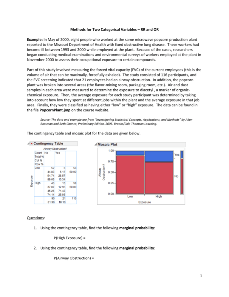
Methods for Two Categorical Variables – RR and OR
Example: In May of 2000, eight people who worked at the same microwave popcorn production plant
reported to the Missouri Department of Health with fixed obstructive lung disease. These workers had
become ill between 1993 and 2000 while employed at the plant. Because of the cases, researchers
began conducting medical examinations and environmental surveys of workers employed at the plant in
November 2000 to assess their occupational exposure to certain compounds.
Part of this study involved measuring the forced vital capacity (FVC) of the current employees (this is the
volume of air that can be maximally, forcefully exhaled). The study consisted of 116 participants, and
the FVC screening indicated that 21 employees had an airway obstruction. In addition, the popcorn
plant was broken into several areas (the flavor-mixing room, packaging room, etc.). Air and dust
samples in each area were measured to determine the exposure to diacetyl , a marker of organicchemical exposure. Then, the average exposure for each study participant was determined by taking
into account how low they spent at different jobs within the plant and the average exposure in that job
area. Finally, they were classified as having either “low” or “high” exposure. The data can be found in
the file PopcornPlant.jmp on the course website.
Source: The data and example are from “Investigating Statistical Concepts, Applications, and Methods” by Allan
Rossman and Beth Chance, Preliminary Edition. 2005. Brooks/Cole Thomson Learning.
The contingency table and mosaic plot for the data are given below.
Questions:
1. Using the contingency table, find the following marginal probability:
P(High Exposure) =
2. Using the contingency table, find the following marginal probability:
P(Airway Obstruction) =
1
3. Using the contingency table, find the joint probability that someone is in the High Exposure
group and has an Airway Obstruction:
P(High Exposure and Airway Obstruction) =
4. Using the contingency table, find the following joint probability:
P(Low Exposure and Airway obstruction) =
5. Using the contingency table, find the following conditional probability. Given that an individual
is in the High Exposure category, what is the probability they have an airway obstruction?
P(Airway Obstruction | High Exposure) =
6. Using the contingency table, find the following conditional probability:
P(Airway Obstruction | Low Exposure) =
Other summaries that are often used when investigating the relationship between categorical variables
are the relative risk and odds ratio.
Relative Risk
Let’s again consider the data from the microwave popcorn plant example.
Low Exposure
High Exposure
Total
Airway Not Obstructed
52
43
95
Airway Obstructed
6
15
21
Total
58
58
106
Note that for these data, P(Airway Obstruction | High Exposure) was more than ___________ as large as
P(Airway Obstruction | Low Exposure). Since this seems like an important feature to describe, we will
compare the two groups using relative risk.
Relative Risk: This is the measure of how much a particular risk factor ________________ the
risk of a specified outcome.
For the popcorn example, we can calculate the relative risk as follows:
RR = Relative Risk =
P(Airway Obstruction | High Exposure)
P(Airway Obstruction | Low Exposure)
=
Proportion with Airway Obstruction in High Exposure Group
Proportion with Airway Obstruction in Low Exposure Group
2
Interpretation of this value:
Comments:
 A relative risk of _____ is the reference value for making comparisons. That is, a relative risk of
_____ says there is _____ difference in the two probabilities.
 The relative risk are easily displayed in the following mosaic plot.
 Alternatively, we could have calculated the relative risk as follows:
RR =
P(Airway Obstruction | Low Exposure)
=
P(Airway Obstruction | High Exposure)
Interpretation: The risk of airway obstruction for the _________ exposure group is _____ times
more likely than the risk of airway obstruction for the _________ exposure
group.
3
Odds Ratio
The relative risk is frequently used when investigating the relationship between two categorical
variables. Although this quantity is relatively easy to calculate and interpret, statisticians often use
another quantity known as an odds ratio in this situation.
Odds: With counts given for two _________ categories (High and Low Exposure), the odds of
“yes” versus “no” is computed as the number of “yes” events versus the number of “no”
events for each group.
Again, let’s consider the microwave popcorn example.
Low Exposure
High Exposure
Total
Airway Not Obstructed
52
43
95
The odds of Airway Obstruction for High =
Airway Obstructed
6
15
21
Total
58
58
106
Number with airway obstruction in High Group
Number with NO airway obstrcution in High Group
=
The Odds of Airway Obstruction for Low =
Number with airway obstruction in Low Group
Number with NO airway obstrcution in Low Group
=
Odds Ratio: This is simply the _________ of the odds for the two groups:
OR = Odds Ratio =
Odds of airway obstruction for High Exposure
Odds of airway obstruction for Low Exposure
Interpretation of this value:
4
We could have also calculated the odds ratio in the following manner:
OR =
Odds of airway obstruction for Low Exposure
Odds of airway obstruction for High Exposure
Interpretation of this value:
Comments:
 An odds ratio of _____ implies there is no observable difference between the two odds.
 The odds can be visualized using the mosaic plot.
5
Relative Risks and Odds Ratios in JMP
We can get these values from JMP using the following directions.
 Once the mosaic plot, contingency table and Tests output has been created by choosing Analyze
 Fit Y by X, click on the little red arrow next to Contingency Analysis of Airway Obstruction? By
Exposure. Then choose Relative Risk.
 The options to choose can be determined from the question or you can ask for all combinations
to be outputted. However, only one of the ratios is most appropriate for each scenario.
 The following output will be given at the bottom of the JMP output window.
 If you check the Calculate all combinations box in the dialogue box given above, you’ll get the
following output.
6
 If you select odds ratio from the same drop-down menu you should get the following output.
Note: JMP always alphabetizes the category names in the contingency table, and then divide the
columns left to right.
OR =
Odds of NO obstruction for Low group
Odds of NO obstruction for the High group
=
Example: According to research reported in the Journal of the National Cancer Institute (April 1991),
eating foods high in fiber may help protect against breast cancer. The researchers randomly divided 120
laboratory rats into two groups of 60 each. All of the rats were injected with a drug that causes breast
cancer. Then each rat was fed a diet of fat and fiber for 15 weeks. However, level of fat and fiber were
varied between the two groups. At the end of the feeding period, the number of rates with cancer
tumors was determined for each group. The data is summarized in the contingency table below.
No Fiber
Fiber
Total
Tumors
46
34
80
No Tumors
14
26
40
Total
60
60
120
Questions:
7. Find the probability a rat had a tumor given they ate a no fiber diet.
8. Find the probability a rate had a tumor given they ate a fiber diet.
9. Find the relative risk of having a tumor for rats who had no fiber compared with those who had
fiber.
7
10. Interpret the relative risk found in Question 9.
11. Using JMP, find and interpret the odds ratio for this scenario.
12. Looking at the relative risk found in Question 9 and the odds ratio found in Question 11, is there
a relationship/association between eating fiber and getting cancer tumors? Explain.
Example: A study was conducted in 1991 by the University of Wisconsin and the Wisconsin Department
of Transportation in which linked police reports and discharge records were used to assess, among other
things, the risk of head injury for motorcyclists in motor-vehicle crashes. The data shown below can be
used to examine the relationship between helmet use and whether brain injury was sustained in the
accident.
Brain Injury
No Brain Injury
Total
Helmet
17
977
994
No Helmet
97
1918
2015
Total
114
2895
3009
Questions:
13. Using JMP, find and interpret the relative risk of brain injury.
8
14. Using JMP, find and interpret the odds ratio.
15. Looking at the relative risk found in Question 13 and the odds ratio found in Question 14, is
there a relationship/association between helmet use and brain injury? Explain.
9