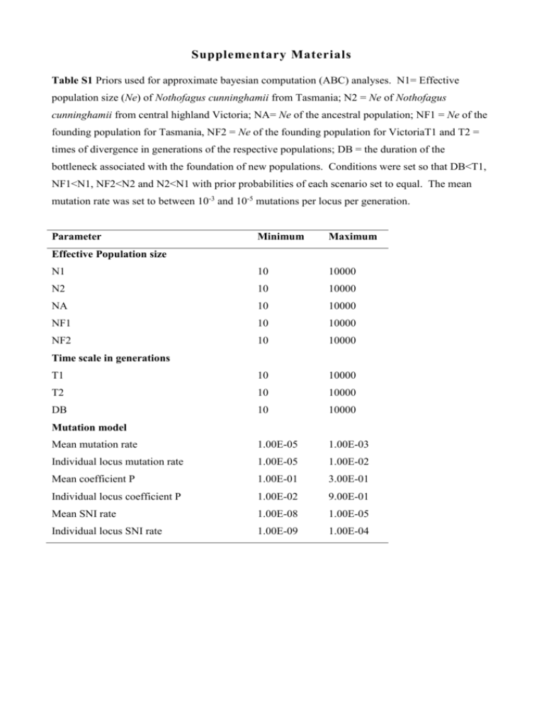
Supplementary Materials
Table S1 Priors used for approximate bayesian computation (ABC) analyses. N1= Effective
population size (Ne) of Nothofagus cunninghamii from Tasmania; N2 = Ne of Nothofagus
cunninghamii from central highland Victoria; NA= Ne of the ancestral population; NF1 = Ne of the
founding population for Tasmania, NF2 = Ne of the founding population for VictoriaT1 and T2 =
times of divergence in generations of the respective populations; DB = the duration of the
bottleneck associated with the foundation of new populations. Conditions were set so that DB<T1,
NF1<N1, NF2<N2 and N2<N1 with prior probabilities of each scenario set to equal. The mean
mutation rate was set to between 10-3 and 10-5 mutations per locus per generation.
Parameter
Minimum
Maximum
N1
10
10000
N2
10
10000
NA
10
10000
NF1
10
10000
NF2
10
10000
T1
10
10000
T2
10
10000
DB
10
10000
Mean mutation rate
1.00E-05
1.00E-03
Individual locus mutation rate
1.00E-05
1.00E-02
Mean coefficient P
1.00E-01
3.00E-01
Individual locus coefficient P
1.00E-02
9.00E-01
Mean SNI rate
1.00E-08
1.00E-05
Individual locus SNI rate
1.00E-09
1.00E-04
Effective Population size
Time scale in generations
Mutation model
Table S2 Results of ABC analyses for estimated historical parameters of Nothofagus cunninghamii
based scenario 3. N1= Effective population size (Ne) of Tasmania; N2 = Ne of central highland
Victoria; t1 = time of divergence in generations; NA= Ne of the ancestral population; µmic_1=
mean mutation rate; pmic = number of repeat motifs added or removed from the microsatellite in
each mutation step and snimic = the single insertion nucleotide rate. Means, medians, modes and
quantiles are given.
Parameter N1
N2
t1
NA
µmic_1
pmic_1
snimic_1
mean
9.31E+03
1.45E+03
2.96E+02
1.27E+03
8.32E-04
2.73E-01 8.22E-06
median
9.50E+03
1.23E+03
2.24E+02
7.21E+02
8.55E-04
2.87E-01 9.86E-06
mode
9.98E+03
9.34E+02
1.67E+02
2.32E+02
1.00E-03
3.00E-01 1.00E-05
q025
7.53E+03
4.03E+02
5.94E+01
5.64E+01
5.32E-04
1.70E-01 5.52E-07
q050
7.98E+03
4.94E+02
7.70E+01
1.00E+02
5.83E-04
1.94E-01 1.35E-06
q250
9.02E+03
8.46E+02
1.49E+02
3.53E+02
7.44E-04
2.62E-01 7.52E-06
q750
9.79E+03
1.73E+03
3.44E+02
1.51E+03
9.43E-04
3.00E-01 1.00E-05
q950
9.97E+03
3.17E+03
7.05E+02
4.48E+03
1.00E-03
3.00E-01 1.00E-05
q975
9.98E+03
4.03E+03
9.05E+02
6.18E+03
1.00E-03
3.00E-01 1.00E-05
Table S3 Mean relative bias of the ABC analyses for estimated historical parameters of Nothofagus
cunninghamii based on the present data sets for scenario 3. Parameters are explained in the caption
for Fig. S1.
Parameter Means
Medians Modes
N1
0.064
0.0689
0.1366
N2
0.088
0.0358
-0.056
t1
0.206
0.119
0.0144
NA
1.273
1.089
0.5872
µmic_1
0.236
0.138
0.0061
pmic_1
0.04
0.0256 -0.0345
snimic_1
14.035
4.2132 -0.7812
Table S3 Posterior probabilities of all 12 scenarios estimated with a maximum of 1% of the simulated datasets. n = the number of simulated datasets
closest to the observed used to estimate the posterior.
Scenario
n
6858
13716
20574
27432
34290
41148
48006
54864
61722
68580
1
0.0042
(0.0000-0.0954)
0.007
(0.0000-0.0667)
0.0098
(0.0000-0.0558)
0.0108
(0.0000-0.0491)
0.0118
(0.0000-0.0454)
0.0123
(0.0000-0.0421)
0.0126
(0.0000-0.0396)
0.013
(0.0000-0.0378)
0.0134
(0.0000-0.0365)
0.0138
(0.0000-0.0356)
2
0.409
(0.2836-0.5345)
0.3932
(0.3034-0.4829)
0.3801
(0.3065-0.4537)
0.3702
(0.3062-0.4342)
0.3648
(0.3072-0.4224)
0.3579
(0.3053-0.4106)
0.3526
(0.3037-0.4014)
0.3483
(0.3026-0.3941)
0.3454
(0.3021-0.3887)
0.343
(0.3019-0.3842)
3
0.3257
(0.2012-0.4501)
0.3645
(0.2831-0.4459)
0.3765
(0.3126-0.4404)
0.383
(0.3271-0.4389)
0.3879
(0.3371-0.4387)
0.3934
(0.3464-0.4404)
0.3969
(0.3530-0.4409)
0.3987
(0.3573-0.4402)
0.3993
(0.3600-0.4387)
0.3993
(0.3618-0.4368)
4
0.0048
(0.0000-0.0960)
0.0064
(0.0000-0.0664)
0.0064
(0.0000-0.0530)
0.0068
(0.0000-0.0458)
0.0069
(0.0000-0.0411)
0.0071
(0.0000-0.0375)
0.0073
(0.0000-0.0348)
0.0076
(0.0000-0.0330)
0.0081
(0.0000-0.0318)
0.0086
(0.0000-0.0309)
5
0.0092
(0.0000-0.0996)
0.0104
(0.0000-0.0699)
0.0121
(0.0000-0.0583)
0.0136
(0.0000-0.0521)
0.0146
(0.0000-0.0484)
0.0151
(0.0000-0.0452)
0.0153
(0.0000-0.0426)
0.0156
(0.0000-0.0407)
0.016
(0.0000-0.0394)
0.0162
(0.0000-0.0383)
6
0.0003
(0.0000-0.0925)
0.0003
(0.0000-0.0613)
0.0004
(0.0000-0.0478)
0.0004
(0.0000-0.0400)
0.0004
(0.0000-0.0353)
0.0005
(0.0000-0.0315)
0.0005
(0.0000-0.0286)
0.0005
(0.0000-0.0265)
0.0006
(0.0000-0.0248)
0.0006
(0.0000-0.0235)
7
0.0786
(0.0000-0.1612)
0.0594
(0.0045-0.1143)
0.0586
(0.0158-0.1014)
0.0587
(0.0229-0.0944)
0.0579
(0.0264-0.0893)
0.0579
(0.0299-0.0859)
0.0583
(0.0328-0.0837)
0.059
(0.0356-0.0825)
0.06
(0.0380-0.0819)
0.0609
(0.0402-0.0817)
8
0.0368
(0.0000-0.1247)
0.0342
(0.0000-0.0926)
0.0342
(0.0000-0.0796)
0.0339
(0.0000-0.0719)
0.0332
(0.0000-0.0666)
0.0326
(0.0029-0.0623)
0.0325
(0.0055-0.0594)
0.0325
(0.0077-0.0574)
0.0319
(0.0087-0.0551)
0.0316
(0.0097-0.0535)
9
0.0395
(0.0000-0.1253)
0.0303
(0.0000-0.0874)
0.0282
(0.0000-0.0726)
0.0275
(0.0000-0.0646)
0.0269
(0.0000-0.0595)
0.0273
(0.0000-0.0562)
0.0277
(0.0015-0.0539)
0.0284
(0.0042-0.0525)
0.0289
(0.0064-0.0514)
0.0293
(0.0081-0.0505)
10
0.0292
(0.0000-0.1166)
0.0269
(0.0000-0.0848)
0.0264
(0.0000-0.0714)
0.0276
(0.0000-0.0651)
0.0273
(0.0000-0.0603)
0.0273
(0.0000-0.0566)
0.0276
(0.0011-0.0541)
0.0277
(0.0033-0.0521)
0.0277
(0.0049-0.0505)
0.0277
(0.0062-0.0492)
11
0.0166
(0.0000-0.1056)
0.0168
(0.0000-0.0756)
0.015
(0.0000-0.0607)
0.014
(0.0000-0.0522)
0.0139
(0.0000-0.0475)
0.0135
(0.0000-0.0434)
0.0132
(0.0000-0.0403)
0.0129
(0.0000-0.0379)
0.0128
(0.0000-0.0362)
0.0128
(0.0000-0.0348)
12
0.046
(0.0000-0.1312)
0.0506
(0.0000-0.1069)
0.0523
(0.0085-0.0962)
0.0535
(0.0167-0.0902)
0.0544
(0.0220-0.0867)
0.0552
(0.0263-0.0840)
0.0555
(0.0293-0.0817)
0.0557
(0.0315-0.0799)
0.056
(0.0333-0.0786)
0.0562
(0.0349-0.0775)
Figure S1 Proportion of membership of clusters identified using Structure assuming 2 clusters.
Note the high incidence of the typically Tasmanian cluster (red) in the two southernmost Victorian
populations. Barriers (predicted with BARRIER version 2.2) to gene flow are indicated by grey
lines; the thickness of the edge of a barrier is proportional to the extent of the barrier and the
adjacent numbers relate to the number of times the barrier was observed across samples.
Figure S2. The 12 scenarios tested for ABC analysis. The colours represent populations that are
either observed (red for Victoria and dark blue for Tasmania) or inferred past populations (other
colours). A change in colour represents formation of a new population.
Figure S3 The partitioning of genetic variance in N. cunninghamii based on (a) 10 loci, and (b) 12
loci. The 10 locus analysis should provide a less biased estimate of the partitioning of variance
because it excludes the two loci with high levels of null alleles, which can cause overestimation of
among individual variance. The levels are: between states, among populations within states, among
subpopulations within populations, among individuals within subpopulations and within individuals,
as identified by AMOVA.
a) Tasmania
0.30
0.25
Fst(1-Fst)
0.20
0.15
0.10
0.05
0.00
0.0
0.5
1.0
-0.05
1.5
2.0
2.5
3.0
2.0
2.5
3.0
Log(1+GGD)
b) Victoria
0.30
0.25
Fst(1-Fst)
0.20
0.15
0.10
0.05
0.00
0.0
0.5
-0.05
1.0
1.5
Log(1+GGD)
Figure S4 Plots of genetic distance versus geographic distance for (a) Tasmanian subpopulations,
and (b) Victorian subpopulations. Mantel tests showed very highly significant associations between
geographic and genetic distances within Victoria both including and excluding the isolated
Kinglake population (P = 0.006 and P<0.001, respectively), but no significant association within
Tasmania (P = 0.125).
(a) Tasmanian Sub Populations
6
Allelic richenss
5
4
3
R² = 0.0183 (not significant; P > 0.05)
2
1
0
0
200
400
600
800
1000
1200
1400
Altitude (m above sea level)
Allelic richness
(b) Victorian Sub Populations
5
4.5
4
3.5
3
2.5
2
1.5
1
0.5
0
R² = 0.0006 (not significant; P > 0.05)
0
200
400
600
800
1000
1200
1400
1600
Altitude (m above sea level)
Figure S5. Relationships between allelic richness (Ar) and altitude of all subpopulations in (a)
Tasmania and (b) Victoria.
Figure S6 Allele frequency histograms showing the count of alleles across all 12 loci within six
allele frequency classes within each of the 18 Nothofagus cunninghamii populations from Tasmania
(a-k) and Victoria (l-r).
Figure S7 The posterior distribution (green lines) and prior distribution (red lines) of the effective
populations size of (a) Tasmanian populations, (b) Victorian populations and (c) the time in
generations of the divergence of these populations. The numbers in brackets are the median values
of the posterior.
a)
b)
c)