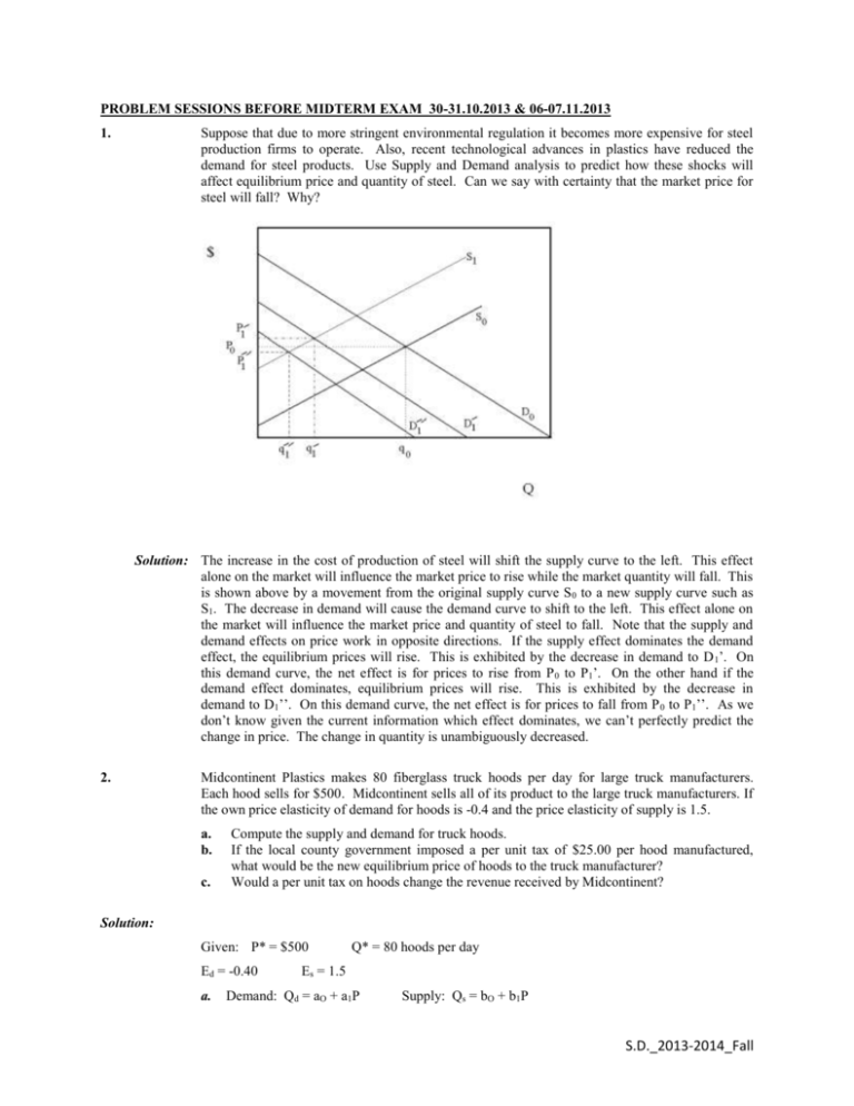
PROBLEM SESSIONS BEFORE MIDTERM EXAM_30-31.10.2013 & 06-07.11.2013
1.
Suppose that due to more stringent environmental regulation it becomes more expensive for steel
production firms to operate. Also, recent technological advances in plastics have reduced the
demand for steel products. Use Supply and Demand analysis to predict how these shocks will
affect equilibrium price and quantity of steel. Can we say with certainty that the market price for
steel will fall? Why?
Solution: The increase in the cost of production of steel will shift the supply curve to the left. This effect
alone on the market will influence the market price to rise while the market quantity will fall. This
is shown above by a movement from the original supply curve S 0 to a new supply curve such as
S1. The decrease in demand will cause the demand curve to shift to the left. This effect alone on
the market will influence the market price and quantity of steel to fall. Note that the supply and
demand effects on price work in opposite directions. If the supply effect dominates the demand
effect, the equilibrium prices will rise. This is exhibited by the decrease in demand to D 1’. On
this demand curve, the net effect is for prices to rise from P 0 to P1’. On the other hand if the
demand effect dominates, equilibrium prices will rise. This is exhibited by the decrease in
demand to D1’’. On this demand curve, the net effect is for prices to fall from P 0 to P1’’. As we
don’t know given the current information which effect dominates, we can’t perfectly predict the
change in price. The change in quantity is unambiguously decreased.
2.
Midcontinent Plastics makes 80 fiberglass truck hoods per day for large truck manufacturers.
Each hood sells for $500. Midcontinent sells all of its product to the large truck manufacturers. If
the own price elasticity of demand for hoods is -0.4 and the price elasticity of supply is 1.5.
a.
b.
c.
Compute the supply and demand for truck hoods.
If the local county government imposed a per unit tax of $25.00 per hood manufactured,
what would be the new equilibrium price of hoods to the truck manufacturer?
Would a per unit tax on hoods change the revenue received by Midcontinent?
Solution:
Given: P* = $500
Ed = -0.40
a.
Q* = 80 hoods per day
Es = 1.5
Demand: Qd = aO + a1P
Supply: Qs = bO + b1P
S.D._2013-2014_Fall
Use: E  P  Q to compute a1 and b1.
Q
P
 0.4 
500
a1
80
1 .5 
a1 = -0.064
500
b1
80
b1 = 0.24
Solve for a0 and b0
b.
Qd = aO + a1P
Q s = b O + b 1P
80 = aO + -0.064(500)
80 = bO + 0.24(500)
ao = 112
bo = -40
Qd = 112 - 0.064P
Qs = -40 + 0.24P
The tax represents a price increase to the purchaser regardless of the current price. Thus, the
supply curve will be adjusted vertically upward by $25.
Qs = -40 + 0.24P or
P
= 166.67 + 4.17 Qs, then
Pt = P + $25 = 166.67 + 25 + 4.17Qs
Pt = 191.67 + 4.17Qs or
Qs = -45.96 + 0.24P
The new equilibrium price will be:
New Supply = Demand
Qs= -45.96 + 0.24P = 112 - 0.064P = Qd
Solving yields P = $519.60 per truck hood
c.
3.
Since the new selling price in (c) is $519.60 and the tax is $25 per hood, Midcontinent
would receive only $494.6 per hood. As quantity sold has fallen too, revenues would
fall.
Suppose that the long-run world demand and supply elasticities of crude oil are -0.906 and
0.515, respectively. The current long-run equilibrium price is $30 per barrel and the equilibrium
quantity is 16.88 billion barrels per year. Derive the linear long-run demand and supply
equations. Next, suppose the long-run supply curve you derived above consists of
competitive supply and OPEC supply. If the long-run competitive supply equation is:
SC  7.78  0.29 P, what must be OPEC's level of production in this long-run equilibrium?
Solution: If the demand curve is linear, it is in the form of QD  a  bP.
Also, we know that
P
Q
 16.88 
E  b    b  E    0.906 
Rearranging the linear expression for
  0.510.
Q
P
 
 30 
 
demand allows us to solve for a as follows: a  QD  bP  a  16.88  0.510(30)  32.180. We
may now write the linear expression for demand as QD  32.18  0.510P. If the supply curve is
linear,
it
is
in
the
form
of
QS  c  dP.
Also,
we
know
that
S.D._2013-2014_Fall
P
Q
 16.88 
E  d    d  E    0.515 
  0.290. Rearranging the linear expression for demand
P
 30 
Q
allows us to solve for c as follows: c  QS  dP  c  16.88  0.290(30)  8.18. We may now
write the linear expression for supply as QS  8.18  0.290P. OPEC's supply is the difference
between the world supply and competitive supply at $30. We know that world supply at $30
is 16.88. Competitive supply at $30 is 7.78  0.29 30  16.48. This implies that OPEC's
supply is 0.4 billion barrels per year at $30 in this long-run equilibrium.
4.
Harding Enterprises has developed a new product called the Gillooly Shillelagh. The market
demand for this product is given as follows:
Q = 240 - 4P
a.
b.
c.
d.
At what price is the price elasticity of demand equal to zero?
At what price is demand infinitely elastic?
At what price is the price elasticity of demand equal to one?
If the Shillelagh is priced at $40, what is the point price elasticity of demand?
Solution:
The demand curve given in this problem is linear. The intercepts of the inverse demand curve on
the price and quantity axes are $60 and 240 respectively. The price elasticity of demand varies
along the length of this demand curve. Demand is infinitely elastic at the intercept on the price
axis. Demand is completely inelastic at the intercept on the quantity axis. Demand is unit
elastic at the half-way point between these two extremes.
a.
Thus, the price elasticity of demand equals zero (is completely inelastic) at a price of zero.
b.
c.
Demand is infinitely elastic at a price of $60.
The price elasticity of demand equals one at a price of $30.
 P   Q 
 Q 
The price elasticity of demand equals   
 . If P equals $40, Q equals 80. 
 is
Q

P

 P 
 
constant along a linear demand curve. In this case it equals -4. Therefore, the price elasticity
of demand equals (40/80)(-4) = -2.
d.
5.
Suppose that a small market Major League Baseball team currently charges $12 for a ticket. At
this price, they are able to sell 12,000 tickets to each game. If they raise ticket prices to $15, they
would sell 11,053 tickets to each game. What is the price elasticity of demand at $12? If the
demand curve is linear, what is the algebraic expression for demand?
Solution:
 P   Q   12   947 
The price elasticity of demand is E    

  0.316. If the

 Q   P   12, 000   3 
demand curve is linear, it is in the form of
QD  a  bP.
P
Q
 12, 000 
E  b    b  E    0.316 
  316.
P
 12 
Q
Rearranging the linear expression for
Also, we know that
demand allows us to solve for a as follows: a  QD  bP  a  12,000  316(12)  15,792. We
may now write the linear expression for demand as QD  15,792  316P.
S.D._2013-2014_Fall
6.
The U.S. Department of Agriculture is interested in analyzing the domestic market for corn. The
USDA's staff economists estimate the following equations for the demand and supply curves:
Qd = 1,600 - 125P
Qs = 440 + 165P
Quantities are measured in millions of bushels; prices are measured in dollars per bushel.
a.
b.
c.
Calculate the equilibrium price and quantity that will prevail under a completely free market.
Calculate the price elasticities of supply and demand at the equilibrium values.
The government currently has a $4.50 bushel support price in place. What impact will this
support price have on the market? Will the government be forced to purchase corn under a
program that requires them to buy up any surpluses? If so, how much?
Solution:
a.
Set Qd = Qs to determine price.
1600 - 125P = 440 + 165P
1160 = 290P
P=4
Obtain Q by substituting into either expression.
Qd = 1600 - 125(4)
Qd = 1600 - 500
Q = 1100
P* = $4, Q* = 1100
b.
c.
For the Own Price Elasticity of Demand E  125 
4
 0.45 (approximately)
1100
For the Own Price Elasticity of Supply E  165 
4
 0.60
1100
Calculate Qd and Qs at the $4.50 price
Qd = 1600 - 125(4.5)
Qd = 1037.5
Qs = 440 + 165(4.5)
Qs = 1182.5
surplus = Qs - Qd = 1182.5 - 1037.5 = 145
The support price would create an excess supply of 145 million bushels that the
government would be forced to buy.
7.
The current price charged by a local movie theater is $8 per ticket. The concession stand at the
theater averages $5 in revenue for each ticket sold. At the current ticket price, the theater typically
sells 300 tickets per showing. If the theater raises ticket prices to $9, the theater will sell 270
S.D._2013-2014_Fall
tickets. What is the price elasticity of demand at $8? What happens to ticket revenue if the theater
increases ticket prices to $9 from $8? What happens to concession revenue if the theater increases
ticket prices? If the theater wants to maximize the sum of ticket and concession revenue, should
they raise ticket prices to $9?
 P   Q   8  30 
Solution: The price elasticity of demand at $8 is E   


  0.8. Initially, ticket
 Q   P   300  1 
revenue is P*Q = $8(300) = $2,400. If ticket prices are raised to $9, ticket revenue becomes P*Q
= $9(270) = $2,430. Thus, if ticket prices are raised to $9, ticket revenue increases by $30. At $8,
the concession stand will average $1,500 per movie showing. If ticket prices are raised to $9, the
concession stand will average $1,350. Thus, concession stand revenues will fall on average by
$150. If the theater wants to maximize the sum of ticket and concession revenue, they should
not raise ticket prices to $9.
8. Donald derives utility from only two goods, carrots (Q c) and donuts (Qd). His utility function is as follows:
U(Qc,Qd) = (Qc)(Qd)
The marginal utility that Donald receives from carrots (MUc) and donuts (MUd) are given as follows:
MUc = Qd
MUd = Qc
Donald has an income (I) of $120 and the price of carrots (Pc) and donuts (Pd) are both $1.
a. What is Donald's budget line?
b. What is Donald's income-consumption curve?
c. What quantities of Qc and Qd will maximize Donald's utility?
d. Holding Donald's income and Pd constant at $120 and $1 respectively, what is Donald's demand curve for
carrots?
e. Suppose that a tax of $1 per unit is levied on donuts. How will this alter Donald's utility maximizing market
basket of goods?
f.
Suppose that, instead of the per unit tax in (e), a lump sum tax of the same dollar amount is levied on Donald.
What is Donald's utility maximizing market basket?
g. The taxes in (e) and (f) both collect exactly the same amount of revenue for the government, which of the two
taxes would Donald prefer? Show your answer numerically and explain why Donald prefers the per unit tax
over the lump sum tax, or vice versa, or why he is indifferent between the two taxes.
S.D._2013-2014_Fall
Solution:
a.
Budget line: 120 = Qc + Qd
b.
The income consumption curve must satisfy:
MUd/MUc = Pd/Pc
Substituting for MUd, MUc, Pd, and Pc yields:
Qc/Qd = 1 or Qc = Qd
c.
Substituting the information in (b) into the budget line:
120 = Qc + Qc = 2Qc
Qc = 60
Qd = 60
d.
Rewriting the budget line:
120 = PcQc + Qd
Substituting the information in (b) into the budget line:
120 = PcQc + Qc = Qc(Pc + 1)
Qc = 120/(Pc + 1)
e.
The $1 tax on donuts raises the after-tax price to $2. The income-consumption curve becomes:
MUd/MUc = Pd/Pc
Substituting for MUd, MUc, Pd and Pc yields:
Qc/Qd = 2 or Qc = 2Qd
The budget line is:
120 = Qc + 2Qd
Substitute the income-consumption curve into the budget line to eliminate Qc:
120 = 2Qd + 2Qd = 4Qd
Qd = 30
Qc = 60
S.D._2013-2014_Fall
f.
Donald buys 30 donuts, so he pays $30 in tax. If Donald paid $30 in a lump sum tax, his income
would be $90. Resolve the utility maximization problem with I = 90, Pc = Pd = 1.
The utility maximizing market basket is Qc = Qd = 45.
g.
Donald prefers the lump-sum tax to the excise tax. Use the utility function to show which market
basket is preferred.
U(Qc, Qd) = QcQd
lump-sum tax
U(45, 45) = 45 x 45 = 2,025
excise tax
U(60, 30) = 60 x 30 = 1,800
9. Using the method of Lagrange multipliers
Each day Paul, who is in third grade, eats lunch at school. He only likes Twinkies (T) and Orange Slice (S), and
these provide him a utility of
𝑈𝑡𝑖𝑙𝑖𝑡𝑦 = 𝑈(𝑇, 𝑆) = √𝑇𝑆
a. If Twinkies cost $.10 each and Slice cost $.25 per cup, how should Paul spend the $1 his mother gives him in
order to maximize his utility?
b. If the school tries to discourage Twinkie consumption by raising the price to $.40, by how much will Paul’s
mother have to increase his lunch allowance to provide him with the same level of utility he received in part (a)?
How many Twinkies and cups of Slice will he buy now (assuming that it is possible to purchase fractional amounts
of both of these goods)?
Solution:
a.
ℒ = 𝑇 0.5 𝑆 0.5 + 𝜆(𝐼 − 𝑃𝑇 𝑇 − 𝑃𝑆 𝑆)
𝜕ℒ
= 0.5𝑇 −0.5 𝑆 0.5 − 𝜆𝑃𝑇 = 0
𝜕𝑇
𝜕ℒ
= 0.5𝑆 −0.5 𝑇 0.5 − 𝜆𝑃𝑆 = 0
𝜕𝑆
𝜕ℒ
= 𝐼 − 𝑃𝑇 𝑇 − 𝑃𝑆 𝑆 = 0
𝜕𝜆
𝑆 𝑃𝑇 0,10
=
=
𝑇 𝑃𝑆 0,25
5𝑆 = 2𝑇
1 = 0.10𝑇 + 0.25𝑆
𝑆=2
𝑇=5
b.
𝑻𝑺 = 𝟏𝟎
𝑆 𝑃𝑇′ 0,40
=
=
𝑇 𝑃𝑆 0,25
S.D._2013-2014_Fall
5𝑆 = 8𝑇
𝑆′ = 4
𝑇 ′ = 5/2
5
𝐼 ′ = 0.40 ( ) + 0.25.4 = 2
2
10. The demand curves for steak, eggs, and hot dogs are given in the table below. The current price of steak is $5.
The price of eggs is $2.50, and the price of hot dogs is $0.75. Fill in the remaining columns of the table using this
information. Indicate which goods are substitutes and which goods are complements.
Good
Steak
Egg
Hotdog
Demand Equation
DS  500  2 PS 
Egg Price
Elasticity of
Demand
Hotdog Price
Elasticity of
Demand
Steak Price
Elasticity of
Demand
Egg Price
Elasticity of
Demand
Hotdog Price
Elasticity of
Demand
1
1
PE 
PH
10
100
DE  75  3PE  PS 
DH  300 
Steak Price
Elasticity of
Demand
1
PH
10
1
1
PH  PS  PE
2
10
Solution:
Good
Steak
Egg
Hotdog
Demand Equation
DS  500  2 PS 
1
1
PE 
PH
10
100
DE  75  3PE  PS 
DH  300 
1
PH
10
1
1
PH  PS  PE
2
10
-0.020
-0.00051
1.53
-0.079
-0.24
1.20E-4
0.016
0.00082
-0.0012
Steak and eggs are complements. Steak and hotdogs and eggs and hotdogs are substitutes.
S.D._2013-2014_Fall
11. Answer both parts of the following question.
a.
b.
The San Francisco Chronicle reported that the toll on the Golden Gate Bridge was raised from $2 to $3.
Following the toll increase, traffic fell by 5 percent. Based on this information, calculate the point price
elasticity of demand. Is demand elastic or inelastic? Explain.
Stephen Leonoudakis, chairman of the bridge's finance auditing committee, warned that the toll increase could
cause toll revenues to decrease by $2.8 million per year. Is this statement consistent with economic theory?
Explain.
Solution:
a.
Increasing the toll on the bridge form $2 to $3 is a 50 percent increase. Traffic is expected to
decrease by 5 percent as a result of the toll increase. Therefore, the point price elasticity of demand
is -5/50 or -0.1. Demand is inelastic.
b.
Stephen Leonoudakis' statement is not consistent with economic theory. When demand is inelastic,
an increase in price will increase total expenditures on a good (the total expenditure on the good is
the total revenue of the firm). Since demand is inelastic here, toll revenues will increase rather than
decrease.
12. The wheat market is perfectly competitive, and the market supply and demand curves are given by the following
equations:
QD = 20,000,000 - 4,000,000P
QS = 7,000,000 + 2,500,000P,
where QD and QS are quantity demanded and quantity supplied measured in bushels, and P = price per bushel.
a. Determine consumer surplus at the equilibrium price and quantity.
b. Assume that the government has imposed a price floor at $2.25 per bushel and agrees to buy any resulting
excess supply. How many bushels of wheat will the government be forced to buy? Determine consumer surplus
with the price floor.
Solution:
a.
The first step is to determine the equilibrium price
 Pe  and quantity Qe  by equating QD and
QS.
20,000,000  4,000,000 Pe  7,000,000  2,500,000 Pe
13,000,000  6,500,000Pe
Pe  $2.00.
Substitute into QD or QS
Qe  20,000,000  4,000,000  2
Qe  12,000,000.
To find consumer surplus, we must also determine the choke price ( PC ). That is, the price at
which quantity demanded is zero. solve for P in terms of QD and QS.
0  20,000,000  4,000,000 PC
4,000,000 PC  20,000,000
PC  5.
S.D._2013-2014_Fall
CS 
1
 PC  Pe  Qe  0.5  5  2 12, 000, 000  18, 000, 000.
2
b.
At price of 2.25
QD = 20,000,000 - 4,000,000(2.25)
QD = 11,000,000
QS = 7,000,000 + 2,500,000(2.25)
QS = 12,625,000
Excess supply is QS - QD.
12,625,000 - 11,000,000 = 1,625,000
Government should expect to buy 1,625,000 bushels.
Cs = (0.5)(Pc-$2.25)QD = (0.5)(5-2.25)(11,000,000)=15,125,000.
C.S. fell from 18,000,000 to 15,125,000
S.D._2013-2014_Fall
13. The following table gives the current price, quantity, and price elasticities of the linear demand curves for
pencils, paper and scissors.
The columns Erc under the Price Elasticities heading are calculated as
 Qr  Pc
Erc  
 . The terms r and c refer to the row of the table and the column under the price elasticities heading,
 Pc  Qr
respectively. For example, if r is one and c is two, the value E12 is the responsiveness of pencil demand to changes
in the paper price (i.e., a cross-price elasticity). The demand curves for each good are in the form
Qr  ar  br P1  cr P2  dr P3 . Using the information in the table, derive the demand curve for each good.
Price Elasticities
Demand Item
Own Price
Quantity
Er 1
Er 2
Er 3
Pencils
0.35
25,000
-1.2
0.25
0
Paper
2.00
90,000
0.01
-0.85
0.45
Scissors
3.15
1,500
0
1.20
-1.75
Solution: Using the information in the table allows us to solve for the coefficients on prices as follows:
Q
br  Er1  r
 P1
 Qr

 ; cr  Er 2 
 P2

equation allows us to solve for
calculations
for
the
 Qr 

 ; and dr  Er 3   . Substituting these coefficient values into the demand

 P3 
ar . This is done by setting ar  Qr   br P1  cr P2  dr P3  . Performing these
first
row
of
the
table
gives
us
the
demand
for
pencils
Q1  48,750  85,714.3P1  3,125P2  0P3 . The demand for paper is Q2 = 125,000 + 2,571.43P1 – 38,250P2
+ 12,857.14P3. The demand for scissors is Q3  2,325  0 P1  900 P2  833.33P3 .
-----------------------------------------------------------------------------------------------------------------------------------------14.
The demand for hamburgers is estimated from this theoretical model:
Q = kPaIbAce,
where Q = units per day, P = price per unit, A = advertising budget per month by sellers, I = per
capita income of consumers, and e = a random error. In a recent study, one researcher estimated
the log-linear form of this equation with regression analysis as:
log Q = 2.5 - 0.33log P + 0.15log I + 0.2log A.
Explain what the coefficients of log P, log I, and log A reveal about this product.
Solution:
The coefficients of the variables are the respective elasticities of demand. The price elasticity is (0.33), income elasticity is 0.15, and advertising elasticity is 0.2. These coefficients indicate that
the product is relatively price inelastic, is a normal good, and is responsive to advertising outlays
by sellers.
S.D._2013-2014_Fall
Adriana is in charge of setting the price on basketball tickets for the local team’s home games.
From previous experience, she has estimated demand to be
15.
P = 50 - 0.00166Q,
where P represents price in dollars per seat, and Q represents seats that could be sold per game.
The seating capacity is 25,000 seats. Determine the number of tickets that would be sold at a
ticket price of $15 each. Also, determine the consumer surplus that could be absorbed from these
consumers if Adriana were able to set ticket prices so that each customer (who values the
ticket at least at $15) pays the entirety of his or her actual valuation of the ticket.
Solution:
50  15
0
At P = 15, the quantity sold is .00166 = 21,084 tickets.
The consumer surplus that could be absorbed is represented by the area under demand and above
the price line at 15. Area = (1/2)b*h.
b = 21,084 - 0 = 21,084
h = 50 - 15 = 35
Consumer surplus = (.5)(21,084)(35) = $368,970
16.
May enjoys spending her free time with her friends at the mall and solving problems from her
microeconomics text. She has 16 hours per week of free time. Diagram May's time constraint. If
1
3
3  P 4
1  F 4
MU F    and MU P    where F is her time spent with friends at the mall and P is
4 F 
4 P 
her time spent working problems, how much time should May spend at each activity?
Solution:
The time constraint is 16 = F + P.
Since the price of each activity is equivalent, May's optimal choice will be to set the marginal
utilities of each activity to be equal. Doing so will allow us to solve for time spent with
friends as a function of time spent working problems.
1
3
3  P 4 1  F 4
MU F        MU P  F  3P. From May's time constraint, we know that
4 F 
4 P 
16  F  P. Substituting the optimal choice of F as a function of P into the time constraint
P4
gives us 16  4 P 
.
F  12
17.
a. On a given evening J.P. Enjoys the consumption of cigars (C) and brandy (B) according to the
function
U(C, B)=20C-C2+18B-3B2
How many cigars and glasses of brandy does he consume during an evening? (Cost is no object to
J.P.)
S.D._2013-2014_Fall
b. Lately, however, J.P. has been advised by this doctors that he should limit the sum of brandy
and cigars consumed to 5. How many glasses of brandy and cigars will he consume under
these circumstances?
Solution:
a.
𝑴𝑼𝑪 =
𝝏𝑼
= 𝟐𝟎 − 𝟐𝑪 = 𝟎
𝝏𝑪
𝑴𝑼𝑩 =
𝝏𝑼
= 𝟏𝟖 − 𝟔𝑩 = 𝟎
𝝏𝑩
𝑪 = 𝟏𝟎
𝑩=𝟑
b.
𝑩+𝑪 =𝟓
S.D._2013-2014_Fall