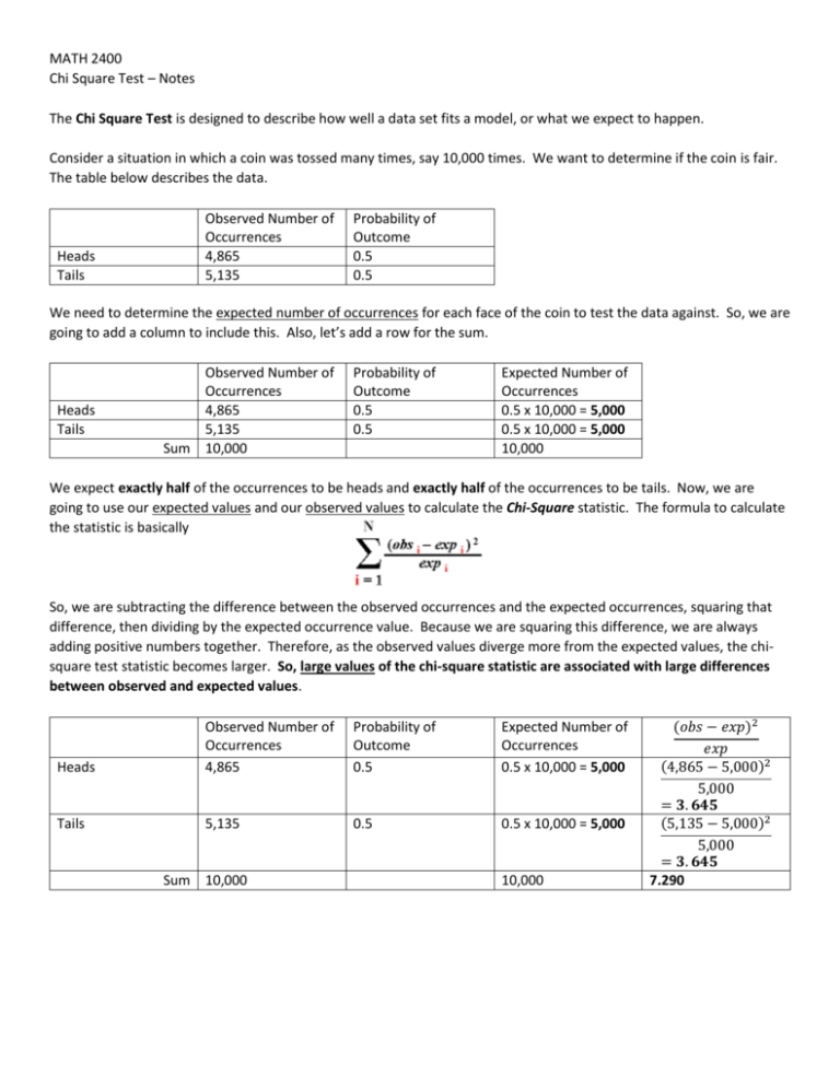
MATH 2400
Chi Square Test – Notes
The Chi Square Test is designed to describe how well a data set fits a model, or what we expect to happen.
Consider a situation in which a coin was tossed many times, say 10,000 times. We want to determine if the coin is fair.
The table below describes the data.
Heads
Tails
Observed Number of
Occurrences
4,865
5,135
Probability of
Outcome
0.5
0.5
We need to determine the expected number of occurrences for each face of the coin to test the data against. So, we are
going to add a column to include this. Also, let’s add a row for the sum.
Heads
Tails
Observed Number of
Occurrences
4,865
5,135
Sum 10,000
Probability of
Outcome
0.5
0.5
Expected Number of
Occurrences
0.5 x 10,000 = 5,000
0.5 x 10,000 = 5,000
10,000
We expect exactly half of the occurrences to be heads and exactly half of the occurrences to be tails. Now, we are
going to use our expected values and our observed values to calculate the Chi-Square statistic. The formula to calculate
the statistic is basically
So, we are subtracting the difference between the observed occurrences and the expected occurrences, squaring that
difference, then dividing by the expected occurrence value. Because we are squaring this difference, we are always
adding positive numbers together. Therefore, as the observed values diverge more from the expected values, the chisquare test statistic becomes larger. So, large values of the chi-square statistic are associated with large differences
between observed and expected values.
Heads
Observed Number of
Occurrences
4,865
Probability of
Outcome
0.5
Expected Number of
Occurrences
0.5 x 10,000 = 5,000
Tails
5,135
0.5
0.5 x 10,000 = 5,000
Sum 10,000
10,000
(𝑜𝑏𝑠 − 𝑒𝑥𝑝)2
𝑒𝑥𝑝
(4,865 − 5,000)2
5,000
= 𝟑. 𝟔𝟒𝟓
(5,135 − 5,000)2
5,000
= 𝟑. 𝟔𝟒𝟓
7.290
Let’s write our null and alternate hypotheses.
H0: The coin is fair
Ha: The coin is not fair
Let’s use an α=0.05 significance level.
If we get p < 0.05, then that is strong evidence against that null which we could say that the evidence suggests the coin is
not fair.
If we get p > 0.05, then that is not sufficient evidence against the null. We could then say that we fail to reject the null.
This would mean that there is not sufficient evidence to suggest that the coin is not fair.
We see that we get a Chi-Square statistic of 7.290. We are dealing with 1 degree of freedom, so, looking at our ChiSquare table of values, we see that a value of 7.290 with 1 degree of freedom has a p-value between .005 and .01.
Since p < 0.05, there is evidence against the null. So, we reject the null hypothesis and state that evidence suggests that
the coin is not fair.
Ex. 1: Consider a situation in which there are 110 houses in a particular neighborhood. Liberals live in 25 of them,
moderates in 55 of them, and conservatives in the remaining 30. An airplane carrying 65 lb. sacks of flour passes over
the neighborhood. For some reason, 20 sacks fall from the plane, each miraculously slamming through the roof of a
different house. None hit the yards or the street, or the land in trees, or anything like that. Each one slams through a
roof. Anyway, 2 slam through a liberal roof, 15 slam through a moderate roof, and 3 slam through a conservative roof.
Should we reject the hypothesis that the sacks of flour hit houses at random?
Observed
Liberal
Moderate
Conservative
Total
Expected
(𝑜𝑏𝑠 − 𝑒𝑥𝑝)2
𝑒𝑥𝑝
Ex. 2: Consider a survey of 100 individuals to determine if they can roll their tongue or not. It is known that this is a
dominant trait, so using a Punnett square, we can determine that 75% of people should be able to roll their tongue and
25% of people should not be able to roll their tongue. The table below describes the survey data.
(𝑜𝑏𝑠 − 𝑒𝑥𝑝)2
Observed
Expected
𝑒𝑥𝑝
Tongue Rollers
90
75
Non-Rollers
10
25
Total
Determine if the data is a good fit by running a Chi-Square test.
Chi-Square Tests for situations involving more than one categorical variable have to be done a little differently.
- The degrees of freedom is calculated by
DF = (r – 1) * (c – 1)
where r is the number of levels for one categorical variable, and c is the number of levels for the other categorical
variable.
- The expected frequencies are computed separately for each level of one categorical variable at each level of the other
categorical variable.
𝑛𝑟 ∙ 𝑛𝑐
𝐸𝑟,𝑐 =
𝑛
where Er,c is the expected frequency count for level r of Variable A and level c of Variable B, nr is the total number of
sample observations at level r of Variable A. nc is the total number of sample observations at level c of Variable B, and n
is the total sample size.
- The Chi-Square test statistic is calculated using the following equation.
2
(𝑂𝑟,𝑐 − 𝐸𝑟,𝑐 )
𝑋 =∑
𝐸𝑟,𝑐
where Or,c is the observed frequency count at level r of Variable A and level c of Variable B, and Er,c is the expected
frequency count at level r of Variable A and level c of Variable B.
2
Ex. 3: A public opinion poll surveyed a simple random sample of 1000 voters. Respondents were classified bygenter and
by voting preference. Results are shown below.
Is there a gender gap? Do the men’s voting preferences differ significantly from the women’s preferences? Use a 0.05
level of significance.
1. State the null and alternate hypotheses.
H0: Gender and voting preferences are independent.
Ha: Gender and voting preferences are not independent.
2. Calculate the degrees of freedom.
DF = (r – 1) * (c – 1) = (2 – 1) * (3 – 1) = 1 * 2 = 2
3. Calculate the expected frequencies.
E1,1 = (400 * 450) / 1000 = 180000/1000 = 180
E1,2 = (400 * 450) / 1000 = 180000/1000 = 180
E1,3 = (400 * 100) / 1000 = 40000/1000 = 40
E2,1 = (600 * 450) / 1000 = 270000/1000 = 270
E2,2 = (600 * 450) / 1000 = 270000/1000 = 270
E2,3 = (600 * 100) / 1000 = 60000/1000 = 60
Which, we can now organize into a new Expected Frequencies Table
4. Calculate the X2 value.
Χ2 = Σ [ (Or,c - Er,c)2 / Er,c ]
Χ2 = (200 - 180)2/180 + (150 - 180)2/180 + (50 - 40)2/40
+ (250 - 270)2/270 + (300 - 270)2/270 + (50 - 60)2/60
Χ2 = 400/180 + 900/180 + 100/40 + 400/270 + 900/270 + 100/60
Χ2 = 2.22 + 5.00 + 2.50 + 1.48 + 3.33 + 1.67 = 16.2
5. Now, compare this value to the value on the table.
Our value for the X2 statistic gives us a value that produces a very small p-value. So, because p
< 0.05, we reject the null hypothesis. There appears to be a relationship between gender and
voting preference.
Ex. 4: Let’s consider all 190 Three Stooges films and two categories. One category is “the role of the third stooge.”
(Curly/Shemp/Joe) and the other is “number of slaps in the film” (which we break into intervals as [0,10], [11,20], [21,
30], [31, 40], [41, ∞)). Notice that both of these are in fact categorical variables, even though “number of slaps in the
film could be dealt with as a quantitative variable. The data can be put in a two-way table as follows.
Perform a X2 test on H0: there is no relationship between the two categorical variables.
1. The null hypothesis has already been stated, state the alternate hypothesis.
2. Calculate the degrees of freedom.
3. Calculate the expected frequencies.
4. Calculate the X2 test statistic.
5. Finally, compare this value to the value on the table. Determine if we should reject the null hypothesis or fail to
reject the null hypothesis.
HOMEWORK PROBLEMS
1. Data from patients’ own assessment of their quality of life relative to what it had been before their heart attack (data
from patients who survived at least a year).
Quality of Life
Canada
United States
Much better
75
541
Somewhat better
71
498
About the same
96
779
Somewhat worse
50
282
Much worse
19
65
Total
311
2165
Is there a significant difference between the distributions of these two outcomes?
2. Data from rolling a single six-sided number cube 600 times is below. Determine if the number cube is fair.
Number Rolled Number of Occurrences
1
82
2
111
3
102
4
120
5
85
6
100
3. In a certain town, there are about one million eligible voters. A SRS of 10,000 eligible voters was chosen to study the
relationship between sex and participation in the last election. The results are summarized in the following table.
We want to check whether being a man or a woman (columns) is independent of having voted in the last election
(rows). In other words, is “sex and voting independent?”