S1: Empirical Determination of Initial Population State
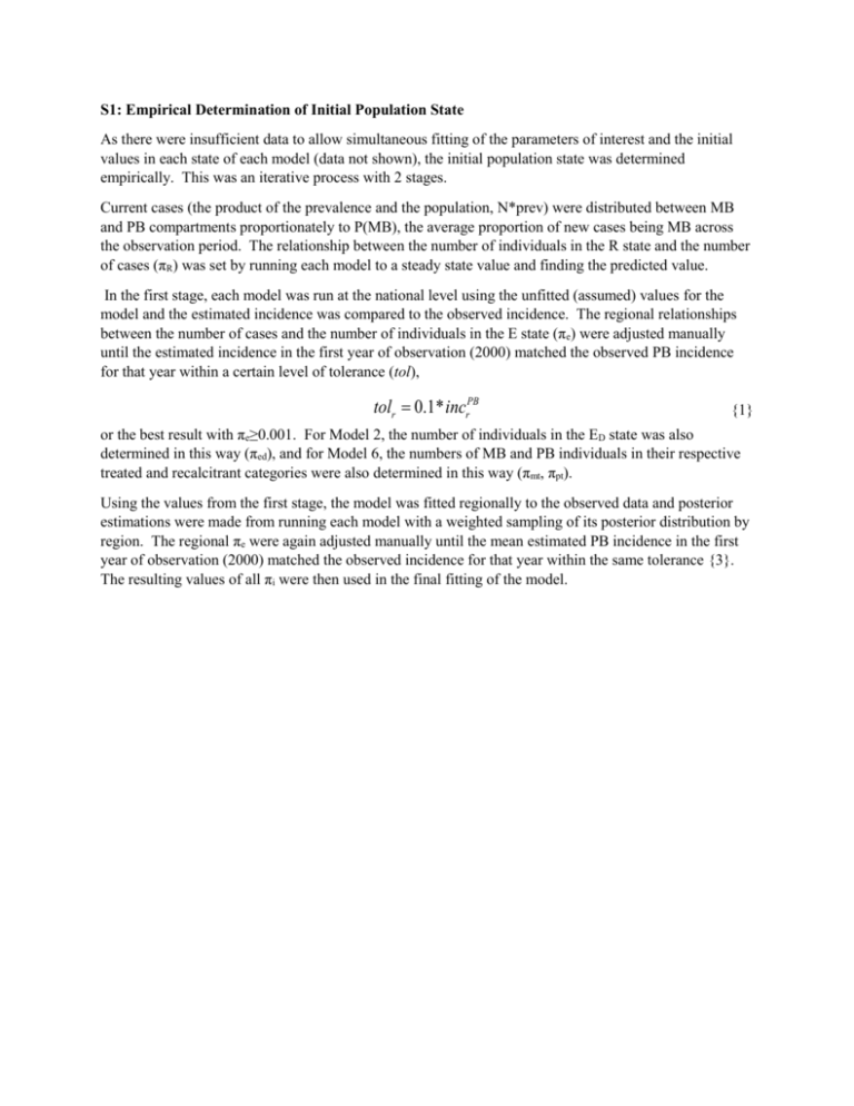
As there were insufficient data to allow simultaneous fitting of the parameters of interest and the initial
values in each state of each model (data not shown), the initial population state was determined
empirically. This was an iterative process with 2 stages.
Current cases (the product of the prevalence and the population, N*prev) were distributed between MB
and PB compartments proportionately to P(MB), the average proportion of new cases being MB across
the observation period. The relationship between the number of individuals in the R state and the number
of cases (πR) was set by running each model to a steady state value and finding the predicted value.
In the first stage, each model was run at the national level using the unfitted (assumed) values for the
model and the estimated incidence was compared to the observed incidence. The regional relationships
between the number of cases and the number of individuals in the E state (πe) were adjusted manually
until the estimated incidence in the first year of observation (2000) matched the observed PB incidence
for that year within a certain level of tolerance (tol),
tolr  0.1* incrPB
{1}
or the best result with πe≥0.001. For Model 2, the number of individuals in the ED state was also
determined in this way (πed), and for Model 6, the numbers of MB and PB individuals in their respective
treated and recalcitrant categories were also determined in this way (πmt, πpt).
Using the values from the first stage, the model was fitted regionally to the observed data and posterior
estimations were made from running each model with a weighted sampling of its posterior distribution by
region. The regional πe were again adjusted manually until the mean estimated PB incidence in the first
year of observation (2000) matched the observed incidence for that year within the same tolerance {3}.
The resulting values of all πi were then used in the final fitting of the model.