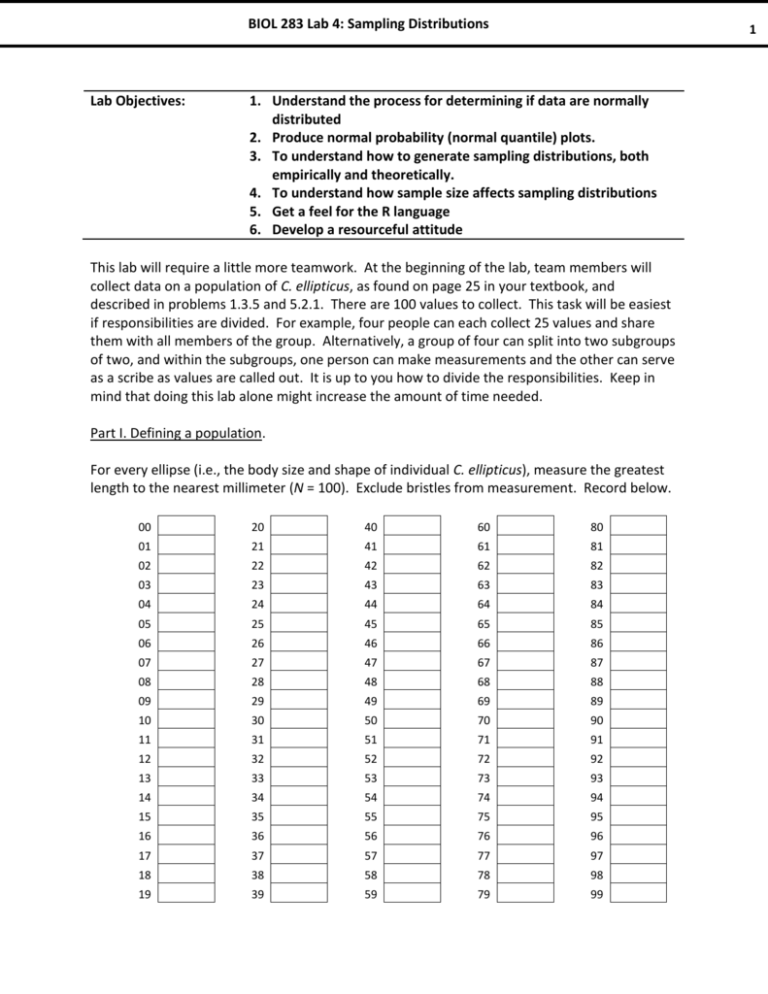
BIOL 283 Lab 4: Sampling Distributions
Lab Objectives:
1
1. Understand the process for determining if data are normally
distributed
2. Produce normal probability (normal quantile) plots.
3. To understand how to generate sampling distributions, both
empirically and theoretically.
4. To understand how sample size affects sampling distributions
5. Get a feel for the R language
6. Develop a resourceful attitude
This lab will require a little more teamwork. At the beginning of the lab, team members will
collect data on a population of C. ellipticus, as found on page 25 in your textbook, and
described in problems 1.3.5 and 5.2.1. There are 100 values to collect. This task will be easiest
if responsibilities are divided. For example, four people can each collect 25 values and share
them with all members of the group. Alternatively, a group of four can split into two subgroups
of two, and within the subgroups, one person can make measurements and the other can serve
as a scribe as values are called out. It is up to you how to divide the responsibilities. Keep in
mind that doing this lab alone might increase the amount of time needed.
Part I. Defining a population.
For every ellipse (i.e., the body size and shape of individual C. ellipticus), measure the greatest
length to the nearest millimeter (N = 100). Exclude bristles from measurement. Record below.
00
20
40
60
80
01
21
41
61
81
02
22
42
62
82
03
23
43
63
83
04
24
44
64
84
05
25
45
65
85
06
26
46
66
86
07
27
47
67
87
08
28
48
68
88
09
29
49
69
89
10
30
50
70
90
11
31
51
71
91
12
32
52
72
92
13
33
53
73
93
14
34
54
74
94
15
35
55
75
95
16
36
56
76
96
17
37
57
77
97
18
38
58
78
98
19
39
59
79
99
BIOL 283 Lab 4: Sampling Distributions
Now create a variable in R for the whole population. This can be done as, for example,
Population = c(y1, y2, y3, …, yN)
Where the values, yi, are data for the variable, Y, which is ellipse length in mm. Make sure you
do this in the exact order of values presented in the table! Note that in R, one can use multiple
lines for one command. This might make it easier to input data. For example, one can do the
following (values are hypothetical):
Population = c(
5, 6, 5, 12, 4, 3, 9, 10, 11, 8,
4, 9, 8, 6, 7, 12, 11, 4, 7, 9,
….
….
….)
Thus, one can do 10 lines of 10 values, or 5 lines of 20 values, or any combination that makes it
easier to know if you have input all 100 values.
Part II. Collecting a sample from the population.
To sample from the population in R, one can use the sample( ) function. Within the
parentheses, add the variable name first, then a comma, then the sample size. For example,
sample(Population, 20)
draws a random sample of 20 subjects from the population (Note that Population means the
name you gave the population). Note that failure to add sample size means that a random
sample of N will be drawn, which effectively just mixes up the values of the population. It is
wise to give the sample a name, so that you can refer to the data later.
For example,
s.20 = sample(Population, 20)
s.15 = sample(Population, 15)
2
BIOL 283 Lab 4: Sampling Distributions
Randomly sample 10
subjects from the
population, and give it a
name
3
What did R provide as output? Do you know which subjects were
chosen? Do you know their lengths?
Now write down the 10 values in increasing order
i
Value:
1
2
3
4
5
6
7
8
Now calculate the percentiles for each value (refer to text or notes)
i
1
2
3
4
5
6
7
9
10
8
9
10
8
9
10
Percentile:
Now calculate the adjusted percentiles (refer to text or notes)
i
1
2
3
4
5
6
7
Adjusted
Percentile:
Now find the standard deviates for each score, assuming a standard normal distribution
i
z:
1
2
3
4
5
6
7
8
9
10
BIOL 283 Lab 4: Sampling Distributions
Finally, make a normal quantile plot by plotting the observed values (y-axis) versus the
quantiles, a. k. a. standard (normal) deviates (x-axis). You can do this by hand, or if you are
savvy, you might try it in R. If you choose the latter, just delete the box below and add a graph
that you made in R. (Make sure to label axes!)
Do the data from the sample pass the “fat pencil” test? I.e., are they normally distributed? If
not, what can you say about the distribution. (Feel free to use the hist( ) or boxplot( ) functions
in R to attain a better understanding of distributional shape. This is why it was a good idea to
give the sample a name)
Provide a comment
about your assessment
of “normality” from the
data.
4
BIOL 283 Lab 4: Sampling Distributions
R has a short-cut for the analysis you just did. Simply use the function, qqnorm(sample), where
sample means your sample name.
Did you get the same
result using the built in
qqnorm( ) function?
Explain.
5
BIOL 283 Lab 4: Sampling Distributions
Part 2. Creating a sampling distribution.
Before creating a sampling distribution, let’s take a look at the population. Using skills you have
learned in this and prior labs, find the population mean and standard deviation, and comment
on the shape of the distribution (using any plotting options you choose). Note: if you use the
function sd( ), the standard deviation will be wrong, as sd( ) calculates the sample standard
deviation. There are several ways to figure out the population standard deviation. Try to find
your own and check with the instructor to make sure you did it right.
Population parameters:
μ:
σ:
Comment on
distribution of lengths
for the population. Use
graphs if you like. Also
comment on how you
found the population
parameters above.
6
BIOL 283 Lab 4: Sampling Distributions
7
Using the sample of 10 you found before, provide the sample mean and standard deviation in
the table below. Also, repeat the sampling procedure you used to get your sample of 10
subjects, originally, 9 more times to produce a total of 10 sample means and standard
deviations. Add those to the table below. In each iteration, calculate the mean and standard
deviation of sample means for all iterations until that point. For example, in iteration 6
calculate the mean and standard deviation of 6 sample means from 6 iterations; in iteration 7,
do the same for 7 values; etc.
Iteration
y
s
Cumulative mY
(Calculate each time)
Cumulative s Y
(Calculate each time)
1
(original sample)
2
3
4
5
6
7
8
9
10
Now compare mY and s Y to m and s , respectively. What appears to be the relationship
between the population and sampling distribution parameters? How might sample size
contribute to your interpretation?
BIOL 283 Lab 4: Sampling Distributions
8
Compare population
and sampling
distribution parameters.
Are your results
consistent with what
you expect?
Part 3. Determining the effect of sample size
Instead of repeating the previous procedure many times with many sample sizes, download the
companion R script and use it to determine how sample size affects the sampling distribution of
Y . Use the script to fill in the table below, along with your own calculations. Then comment
on how the “Law of Large” numbers and “The Central Limit Theorem” apply to this exercise, as
well as what the resampling experiment demonstrates.
10
permutations
n
mY
sY
50
permutations
mY
sY
100
permutations
mY
sY
500
permutations
mY
sY
1000
permutations
mY
sY
5
10
20
40
You can copy and paste plots at the end of this lab exercise, if it helps you remember the
output for the future.
s
n
BIOL 283 Lab 4: Sampling Distributions
CHALLENGE:
At which points in your
simulation exercise did
you find accurate results
with respect to theory?
What does this tell you
about the “Law of Large
Numbers” and the
“Central Limit Theorem”?
9