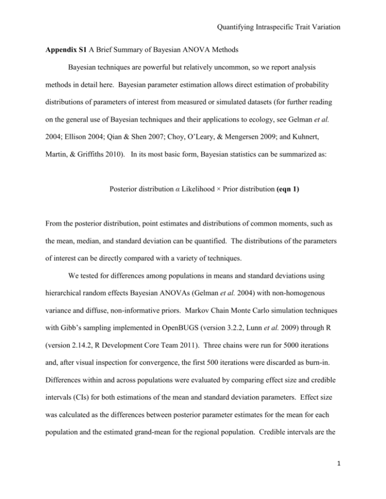
Quantifying Intraspecific Trait Variation
Appendix S1 A Brief Summary of Bayesian ANOVA Methods
Bayesian techniques are powerful but relatively uncommon, so we report analysis
methods in detail here. Bayesian parameter estimation allows direct estimation of probability
distributions of parameters of interest from measured or simulated datasets (for further reading
on the general use of Bayesian techniques and their applications to ecology, see Gelman et al.
2004; Ellison 2004; Qian & Shen 2007; Choy, O’Leary, & Mengersen 2009; and Kuhnert,
Martin, & Griffiths 2010). In its most basic form, Bayesian statistics can be summarized as:
Posterior distribution α Likelihood × Prior distribution (eqn 1)
From the posterior distribution, point estimates and distributions of common moments, such as
the mean, median, and standard deviation can be quantified. The distributions of the parameters
of interest can be directly compared with a variety of techniques.
We tested for differences among populations in means and standard deviations using
hierarchical random effects Bayesian ANOVAs (Gelman et al. 2004) with non-homogenous
variance and diffuse, non-informative priors. Markov Chain Monte Carlo simulation techniques
with Gibb’s sampling implemented in OpenBUGS (version 3.2.2, Lunn et al. 2009) through R
(version 2.14.2, R Development Core Team 2011). Three chains were run for 5000 iterations
and, after visual inspection for convergence, the first 500 iterations were discarded as burn-in.
Differences within and across populations were evaluated by comparing effect size and credible
intervals (CIs) for both estimations of the mean and standard deviation parameters. Effect size
was calculated as the differences between posterior parameter estimates for the mean for each
population and the estimated grand-mean for the regional population. Credible intervals are the
1
Quantifying Intraspecific Trait Variation
95% likelihood of the posterior distribution for a given parameter (i.e. there is a 95% probability
that the parameter lies within that interval). Population effect was considered significant if the
95% CI did not bound zero, which represents no difference from the grand mean. Means for
populations were considered significantly different if their 95% CIs did not overlap.
Significant differences in trait variation were indicated by a lack of overlap in 95% CIs.
Population-level trait distributions were constructed using hyper-parameters estimated in
hierarchical models.
Models
For the ith individual in the jth population, we assume SLA is log-normally distributed with a
population level mean (θj) and population precision term (τ[j]) (where τ = 1/σ2):
:
SLAi,j ~ ln N (θj,τ[j]) i=1,…,nj; j=1,…,10 (eqn 1)
Next, we assume that the population level mean is lognormally distributed with a species-level
mean (µ) and population to population level precision term (τ[j]):
θj~ ln N(µ,τ [j]) j=1,…,10 (eqn 2)
We gave our species level mean µ an uninformative prior:
µ~N(0,1) (eqn 3)
Finally, we gave our population precision terms uninformative priors:
τ[j]~Γ(α, β) (eqn 4)
where:
α ~ U(0,10) (eqn 7)
2
Quantifying Intraspecific Trait Variation
β ~ U(0,10) (eqn 8)
For the ith individual in the jth population, we assume diameter was normally distributed with a
population level mean (θj) and population precision term (τj)
Diameteri,j~N(θj,τ [j]) i=1,…,nj; j=1,…,10 (eqn 9)
Next, we assume that the population level mean is normally distributed with a species-level
mean (µ) and population level precision term (τ [j]):
θj ~N(µ,τ[j]) j=1,…,10 (eqn 10)
We gave our species level mean µ uniformative priors:
µ~N(0,100) (eqn 11)
And our population precision term τ[j] uniformative priors:
τ[j]~Gamma(α, β) (eqn 12)
where:
α ~ U(0.1, 0.1) (eqn 15)
β ~ U(0.1, 0.1) (eqn 16)
Works Cited
Choy, S.L., O’Leary, R. & Mengersen, K. (2009) Elicitation by design in ecology: Using expert
opinion to inform priors for Bayesian statistical models. Ecology, 90, 265–77.
Ellison, A.M. (2004) Bayesian inference in ecology. Ecology Letters, 7, 509–520.
Gelman, A., Carlin, J.B., Stern, H.S. & Rubin, D.B. (2004) Bayesian Data Analysis, 2nd ed (eds
C Chatfield, M Tanner, and J Zidek). Chapman and Hall/CRC, Boca Raton.
Kuhnert, P.M., Martin, T.G. & Griffiths, S.P. (2010) A guide to eliciting and using expert
knowledge in Bayesian ecological models. Ecology Letters, 13, 900–14.
Lunn, D., Spiegelhalter, D., Thomas, A. & Best, N. (2009) The BUGS project: Evolution,
critique and future directions. Statistics in Medicine, 28, 3049–3067.
3
Quantifying Intraspecific Trait Variation
Qian, S.S. & Shen, Z. (2007) Ecological applications of multilevel analysis of variance. Ecology,
88, 2489–95.
R Development Core Team. (2011) R: A Language and Environment for Statistical Computing.
R Foundation for Statitical Computing, Vienna, Austria.
4