1
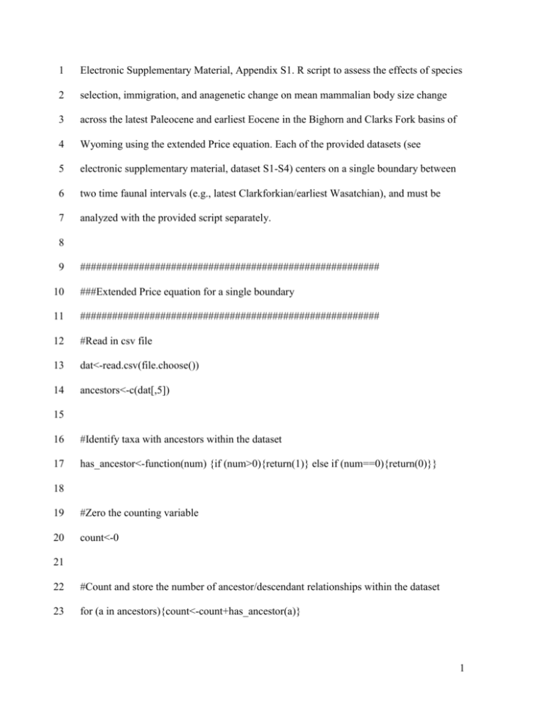
Electronic Supplementary Material, Appendix S1. R script to assess the effects of species
2
selection, immigration, and anagenetic change on mean mammalian body size change
3
across the latest Paleocene and earliest Eocene in the Bighorn and Clarks Fork basins of
4
Wyoming using the extended Price equation. Each of the provided datasets (see
5
electronic supplementary material, dataset S1-S4) centers on a single boundary between
6
two time faunal intervals (e.g., latest Clarkforkian/earliest Wasatchian), and must be
7
analyzed with the provided script separately.
8
9
########################################################
10
###Extended Price equation for a single boundary
11
########################################################
12
#Read in csv file
13
dat<-read.csv(file.choose())
14
ancestors<-c(dat[,5])
15
16
#Identify taxa with ancestors within the dataset
17
has_ancestor<-function(num) {if (num>0){return(1)} else if (num==0){return(0)}}
18
19
#Zero the counting variable
20
count<-0
21
22
#Count and store the number of ancestor/descendant relationships within the dataset
23
for (a in ancestors){count<-count+has_ancestor(a)}
1
24
links<-count
25
26
#Count the number of taxon occurrences (i.e., total number of occurrences in both the
27
#older or younger time intervals)
28
countn<-function(num){length(num[!is.na(num)])}
29
30
#Count the number of descendants in the older time interval and the number of ancestors
31
#in the younger time interval
32
desc_i<-countn(dat[,4])
33
anc_j<-countn(dat[,3])
34
35
#Calculate the mean body size of ancestors and the mean body size of descendants,
36
#omitting missing data
37
mean_anc_size_i<-mean(dat[,3], na.rm=TRUE)
38
mean_desc_size_j<-mean(dat[,4], na.rm=TRUE)
39
40
#Calculate the difference between the mean ancestor and mean descendant sizes
41
xbar_anc_desc<-mean_anc_size_i-mean_desc_size_j
42
43
#Set the index variable to the first column of the dataset
44
index<-c(dat[,1])
45
46
#Calculate the number of ancestors for each taxon
2
47
for (x in index){dat[x, "no_anc"]<-has_ancestor(c(dat[x,5]))}
48
49
#Separate immigrants in dataset
50
dat$no_anc<-ifelse((!is.na(dat$size_i==TRUE)&(dat$ancestor==0)),NA,(dat$no_anc))
51
52
#Calculate the number of descendants for each taxon
53
for (x in index) {if
54
((!is.na(dat[x,"size_i"])==FALSE)&&((!is.na(dat[x,"size_j"])==TRUE)))
55
{dat[x,"no_desc"]<-NA} else {dat[x, "no_desc"]<-nrow(dat[dat$ancestor==x,])}}
56
57
#Restrict the dataset to taxa with ancestors
58
non_missing_ancs<-na.omit(as.numeric(dat[,"no_anc"]))
59
60
#Calculate average number of ancestors, omitting missing data
61
average_ancestors<-mean(non_missing_ancs)
62
63
#Remove taxa with no descendants
64
non_missing_desc<-na.omit(as.numeric(dat[,"no_desc"]))
65
66
#Calculate the average number of ancestors, omitting missing data
67
average_descendants<-mean(non_missing_desc)
68
69
#Calculate relative fitness for each taxon
3
70
for (x in index) {dat[x, "rel_fitness"]<-dat[x,"no_desc"]/average_descendants}
71
72
#Create separate column for ancestor size
73
for (x in index) {if (dat[x,"ancestor"]>0) {dat[x,"anc_size"]<-
74
dat[(dat[x,"ancestor"]),"size_i"]}}
75
76
#Calculate the difference in mean body size between descendants and ancestors
77
dat$size_diff<-dat$size_j-dat$anc_size
78
79
#Calculate the contribution of anagenetic changes (i.e., term three of the extended Price
80
#equation)
81
transmission_bias<-mean(dat$size_diff, na.rm=TRUE)
82
83
#Calculate the difference between the number of descendants in the older time interval
84
#and mean number of descendants per ancestor in the older time interval
85
dat$diff_desc_i_mean<-as.numeric(dat$no_desc) - average_descendants
86
87
#Calculate the difference between the number of ancestors of the younger time interval
88
#and mean number of ancestors per descendant in the younger time interval
89
dat$diff_anc_j_mean<-as.numeric(dat$no_anc) - as.numeric(average_ancestors)
90
91
dat$diff_anc_size_i_mean <-(dat$size_i)-mean_anc_size_i
92
4
93
dat$anc_i_covar_contr<-(dat$diff_desc_i_mean)*(dat$diff_anc_size_i_mean)
94
dat$diff_desc_size_j_mean<-(dat$size_j)-mean_desc_size_j
95
dat$desc_j_covar_contr<-(dat$diff_anc_j_mean)*(dat$diff_desc_size_j_mean)
96
97
#Remove missing data to calculate the covariance of the ancestor contribution
98
nonmissing_covar_anc<-na.omit(as.numeric(dat[,"anc_i_covar_contr"]))
99
100
#Remove missing data to calculate the covariance of the descendant contribution
101
nonmissing_covar_desc<-na.omit(as.numeric(dat[,"desc_j_covar_contr"]))
102
103
#Calculate the contribution of species selection (i.e., term one of the extended Price
104
#equation)
105
covar_term_1<-(sum(nonmissing_covar_anc)/anc_j)/(links/anc_j)
106
107
#Calculate the contribution of immigration (i.e., term two of the extended Price
108
#equation)
109
covar_term_2<-(sum(nonmissing_covar_desc)/desc_i)/(links/desc_i)*-1
110
111
112
113
114
115
5
116
117
Electronic Supplementary Material, Appendix S2.
The three terms of the Price equation are not best thought of as statistical
118
estimates of unknown population parameters. The Price equation does not treat the
119
observed data as sample data, and does not depend on any assumptions about the
120
sampling process (e.g., regarding randomness and independence of observations, the
121
distribution from which the observations were sampled, etc.). Rather, the Price equation
122
takes the observed data as given and reveals what those data imply about the species
123
selection, immigration, and anagenetic change. Rice [1,2] developed a prospective
124
extension of the Price equation in which phenotypes and fitnesses are unknown and so
125
are treated as random variables described by probability distributions; however, this
126
approach does not apply to fossil data describing evolution that has already occurred.
127
Nevertheless, our results are subject to various sources of uncertainty.
128
Quantifying these various sources of uncertainty is desirable in principle but difficult in
129
practice for our dataset. In order to quantify uncertainty in the terms of the Price
130
equation, it would be necessary to quantify sources of error in the observed data, and then
131
propagate those errors through the Price equation. For instance, we estimated the body
132
size of each species as the mean of the natural logarithm of lower first or second molar
133
area. These means are subject to sampling error, with the measured molars of each
134
species being a sample from the population of molars. In principle, this sampling error
135
could be quantified by bootstrapping. Resampling with replacement from the molar
136
measurements of each species would generate bootstrap replicates, each of which could
137
be analyzed with the Price equation, yielding a bootstrapped distribution for each Price
138
equation term. In practice, however, this cannot be accomplished since measurements of
6
139
individual fossils are unavailable for some species, and because some species are known
140
from only a single specimen or only a few specimens at our study site (see electronic
141
supplementary material, table S2). Other sources of error are more difficult to quantify.
142
New fossil discoveries that added new species to our dataset, or altered the timing of
143
species’ first and last appearances would alter our results. So would revisions to species’
144
ancestor-descendant relationships and classification.
145
Assessing whether the observed values of species selection, anagenesis, and non-
146
random immigration across the PETM are different than would be expected under some
147
“null” model with a randomization test is another possibility. However, a biologically-
148
relevant “null” hypothesis is impossible to define. For instance, randomly shuffling body
149
sizes among species and then applying the extended Price equation to the randomized
150
data sets would provide the distribution of results expected under a “null” model in which
151
all species are equally likely to speciate, go extinct, or change in size by any amount. It
152
would not be scientifically informative to either reject this model, or fail to reject it,
153
because this model obviously is biologically implausible. Similarly, randomly shuffling
154
which descendant species descended from which ancestral species would provide the
155
distribution of results expected under an implausible null model in which all ancestor-
156
descendant links are equally probable. In principle, it would be informative to simulate
157
data expected under alternative plausible evolutionary scenarios. The available data,
158
however, are insufficient to guide and constrain development of models of different
159
scenarios.
160
161
7
162
Electronic Supplementary Data, Table S1. Latest Palaeocene and earliest Eocene
163
mammals from the Bighorn and Clarks Fork Basins, Wyoming, USA, studied to examine
164
the macroevolution of mean body size using the extended Price equation. Lineages, with
165
respective sources, are: Palaeanodon [3], Esthonyx [3, unpublished data], Azygonyx [3,4],
166
Macrocranion [4,5, unpublished data], Phenacolemur [6], Niptomomys [4,7], Carpolestes
167
[8,9], Teilhardina [4,10,11], Tetonius [12], Cantius [3,4, unpublished data], Arfia [3],
168
Galecyon [13], Didymictis [14], Viverravus [4,14], Chriacus [3,4], Hyopsodus [15],
169
Haplomylus [16], Phenacodus [4,17], Ectocion [3,4,17], Copecion [17], Diacodexis [3,4,
170
unpublished data], Sifrhippus sandrae/Arenahippus grangeri [3,4,18, unpublished data],
171
and Paramys [19].
172
173
174
175
176
177
178
179
180
181
182
183
184
8
185
Order
?Pholidota
Suborder
Palaeanodonta
Family
Metacheiromyidae
Genus
Palaeanodon
Cimolesta
Tillodonta
Esthonychidae
Esthonyx
Azygonyx
Lipotyphla
Erinaceomorpha
Amphilemuridae
Macrocranion
Primates
Plesiadapiformes
Paromomyidae
Phenacolemur
Microsyopsidae
Carpolestidae
Niptomomys
Carpolestes
Omomyidae
Teilhardina
Notharctidae
Tetonius
Cantius
Creodonta
Hyaenodontidae
Arfia
Carnivora
Viverravidae
Galecyon
Didymictis
Condylarthra
Arctocyonidae
Viverravus
Chriacus
Phenacodontidae
Ectocion
Euprimates
Copecion
Phenacodus
Hyopsodontidae
Hyopsodus
Haplomylus
Artiodactyla
Diacodexeidae
Diacodexis
Perissodactyla
Equidae
Sifrhippus
Arenahippus
Paramys
Rodentia
Sciuromorpha
Ischyromyidae
Species
Palaeanodon parvulus
Palaeanodon nievelti
Esthonyx spatularius
Azygonyx xenicus
Azygonyx anyclion
Azygonyx latidens
Azygonyx grangeri
Azygonyx gunnelli
Azygonyx sp.
Macrocranion junnei
Macrocranion nitens
Phenacolemur pagei
Phenacolemur praecox
Niptomomys doreenae
Carpolestes nigridens
Carpolestes simpsoni
Teilhardina brandti
Teilhardina gingerichi
Teilhardina americana
Tetonius matthewi
Cantius torresi
Cantius ralstoni
Cantius mckennai
Arfia junnei
Arfia zele
Arfia shoshoniensis
Galecyon peregrinus
Didymictis proteus
Didymictis leptomylus
Didymictis protenus
Viverravus politus
Chriacus sp.
Chriacus badgleyi
Ectocion osbornianus
Ectocion parvus
Copecion brachypternus
Copecion davisi
Phenacodus intermedius
Phenacodus trilobatus
Phenacodus vortmani
Hyopsodus loomisi
Haplomylus palustris
Haplomylus simpsoni
Haplomylus zalmouti
Haplomylus speirianus
Diacodexis illicis
Diacodexis metasiacus
Sifrhippus sandrae
Arenahippus grangeri
Paramys taurus
186
187
9
188
Electronic Supplementary Data, Table S2. Mean of the natural logarithm of the first or
189
second molar area (mm) of latest Palaeocene and earliest Eocene mammals from the
190
Bighorn and Clarks Fork Basins, Wyoming, USA, studied to examine the macroevolution
191
of mean body size using the extended Price equation. Sample sizes are provided in
192
parentheses.
193
194
195
196
197
198
199
200
201
202
203
204
205
206
207
208
209
210
10
211
Species
Palaeanodon parvulus
Palaeanodon nievelti
Esthonyx spatularius
Azygonyx xenicus
Azygonyx anyclion
Azygonyx latidens
Azygonyx grangeri
Azygonyx gunnelli
Azygonyx sp.
Macrocranion junnei
Macrocranion nitens
Phenacolemur pagei
Phenacolemur praecox
Niptomomys doreenae
Carpolestes nigridens
Carpolestes simpsoni
Teilhardina brandti
Teilhardina gingerichi
Teilhardina americana
Tetonius matthewi
Cantius torresi
Cantius ralstoni
Cantius mckennai
Arfia junnei
Arfia zele
Arfia shoshoniensis
Galecyon peregrinus
Didymictis proteus
Didymictis leptomylus
Didymictis protenus
Viverravus politus
Chriacus sp.
Chriacus badgleyi
Ectocion osbornianus
Ectocion parvus
Copecion brachypternus
Copecion davisi
Phenacodus intermedius
Phenacodus trilobatus
Phenacodus vortmani
Hyopsodus loomisi
Haplomylus palustris
Haplomylus simpsoni
Haplomylus zalmouti
Haplomylus speirianus
Diacodexis illicis
Diacodexis metasiacus
Sifrhippus sandrae
Arenahippus grangeri
Paramys taurus
Cf1
Cf2
3.09 (2)
Cf3
3.24 (2)
Wa0
Wa1/2
2.80 (2)
3.69 (2)
2.82 (6)
3.77 (27)
4.25 (2)
4.45 (4)
0.68 (3)
4.45 (3)
3.88 (2)
4.03 (2)
4.18 (4)
4.42 (6)
4.72 (5)
0.73 (1)
1.43 (1)
1.01 (7)
1.53 (3)
1.07 (5)
0.85 (4)
1.49 (5)
1.66 (4)
1.78 (1)
0.06 (3)
1.76 (15)
0.40 (6)
0.84 (11)
1.09 (9)
1.29 (1)
1.13 (20)
1.55 (4)
2.32 (3)
2.46 (163)
2.55 (67)
2.88 (4)
3.69 (3)
3.94 (13)
3.98 (9)
3.15 (1)
2.53 (2)
3.01 (1)
2.98 (4)
3.19 (2)
3.59 (37)
3.55 (46)
3.50 (157)
2.89 (1)
3.61 (3)
2.89 (1)
3.19 (3)
3.46 (18)
3.30 (3)
3.79 (13)
4.32 (5)
3.20 (5)
3.16 (2)
2.93 (8)
3.54 (181)
3.17 (35)
3.56 (1)
3.61 (2)
4.77 (10)
4.80 (14)
4.82 (31)
4.39 (2)
4.24 (2)
4.23 (5)
1.82 (6)
1.98 (11)
3.56 (11)
3.20 (4)
4.72 (4)
4.17 (4)
2.10 (33)
4.67 (9)
4.55 (11)
4.07 (20)
2.30 (215)
1.58 (1)
1.17 (7)
1.65 (162)
2.38 (14)
2.55 (174)
3.44 (87)
1.85 (1)
1.93 (2)
1.95 (4)
3.55 (294)
1.89 (1)
212
213
214
11
215
Electronic Supplementary Data, Figure S1. The number of descendant species descended
216
from each ancestral species, as a function of mean ancestral body size, approximated
217
from the natural logarithm of the lower first or second molar area for (a) the early to
218
middle Clarkforkian, (b) middle to late Clarkforkian, (c) late Clarkforkian to earliest
219
Wasatchian, and (d) earliest Wasatchian to early Wasatchian. Each point gives data for
220
one ancestral species. Lines are linear regressions. Insets provide the three
221
subcomponents of species selection (equation 2): the selection gradient (regression slope)
222
β, the variance in body size among ancestral species, σ2, and the mean number of
223
descendant species to which an ancestral species gives rise, 𝑦̅.
224
225
226
227
228
229
230
231
232
233
234
235
236
237
12
3
2
β = -0.14
σ² = 1.67
ӯ = 1. 11
(a)
Carpolestes
1
1
Number of descendants per ancestor
3
2
3
(b)
4
5
Azygonyx
Phenacolemur
2
6
β = 0.14
σ² = 1.46
ӯ = 1. 14
1
1
3
2
3
4
5
6
β = 0.11
σ² = 1.46
Azygonyx ӯ = 0.69
(c)
2
1
Carpolestes
1
3
2
3
4
5
Didymictis
2
6
β = -0.01
σ² = 1.44
ӯ = 0.88
(d)
Cantius
1
1
2
3
4
5
6
Ancestral body size
(mean ln molar area (mm))
238
239
13
240
Electronic Supplementary Data, Figure S2. The number of ancestors for each descendant
241
species, as a function of mean descendant body size, approximated as the natural
242
logarithm of the lower first or second molar area, for (a) the early to middle Clarkforkian,
243
(b) late Clarkforkian to earliest Wasatchian, and (c) earliest Wasatchian to early
244
Wasatchian. The middle to late Clarkforkian boundary is omitted because there was no
245
immigration across this boundary. Each point gives data for one descendant species.
246
Lines are linear regressions. Insets provide the three subcomponents of the effect of non-
247
random immigration (equation 3): the regression slope β, the variance in body size among
248
descendant species, σ2, and the mean number of ancestral species per descendant species,
249
𝑦̅ (equal to the proportion of descendant species that are not immigrants, and so have one
250
ancestor in the dataset).
251
252
253
254
255
256
257
258
259
260
261
262
14
Number of ancestors per descendant
(0 = immigrant, 1 = non-immigrant)
1
(a)
β = 0.02
σ² = 1.46
ӯ = 0.71
1
1
2
3
4
5
6
(b)
β = 0.16
σ² = 1.45
ӯ = 0.46
1
1
2
3
4
5
6
(c)
β = -0.04
σ² = 1.33
ӯ = 0.85
1
2
3
4
5
6
Descendant body size
(mean ln molar area (mm))
263
264
15
265
References
266
267
1. Rice SH. 2008 A stochastic version of the Price equation reveals the interplay of
268
deterministic and stochastic processes in evolution. BMC Evol. Biol. 8, 262.
269
(doi:10.1186/1471-2148-8-262)
270
271
2. Rice SH, Papadopoulos A. 2009 Evolution with stochastic fitness and stochastic
272
migration. PLoS ONE 4, e7130. (doi:10.1371/journal.pone.00007130)
273
274
3. Gingerich PD. 1989 New earliest Wasatchian mammalian fauna from the Eocene of
275
northwestern Wyoming: composition and diversity in a rarely sampled high-floodplain
276
assemblage. Univ. Mich. Pap. Paleontol. 28, 1-97.
277
278
4. Rose KD, Chew AE, Dunn RH, Kraus MJ, Fricke HC, Zack SP. 2012 Earliest Eocene
279
mammalian fauna from the Paleocene-Eocene Thermal Maximum at Sand Creek Divide,
280
southern Bighorn Basin. Univ. Mich. Pap. Paleontol. 36, 1-122.
281
282
5. Bown TM, Schankler D. 1982 A review of the Proteutheria and Insectivora from the
283
Willwood Formation (Lower Eocene), Bighorn Basin, Wyoming. U.S. Geol. Surv. Bull.
284
1523, 1-79.
285
16
286
6. Rose KD. 1981 The Clarkforkian Land Mammal Age and mammalian faunal
287
composition across the Paleocene-Eocene boundary. Univ. Mich. Pap. Paleontol. 26, 1-
288
197.
289
290
7. Bown, T. M. 1979 Geology and mammalian paleontology of the Sand Creek facies,
291
lower Willwood Formation (lower Eocene), Washakie County, Wyoming. Geol. Surv.
292
Wyo. Mem. 2, 1-151.
293
294
8. Bloch JI, Gingerich PD. 1998 Carpolestes simpsoni, new species (Mammalia,
295
Proprimates) from the late Paleocene of the Clarks Fork Basin, Wyoming. Contrib. Mus.
296
Paleontol. Univ. Mich. 30, 131-162.
297
298
9. Bloch JI, Fisher DC, Rose KD, Gingerich PD. 2001 Stratocladistic analysis of
299
Paleocene Carpolestidae (Mammalia, Plesiadapiformes) with description of a new late
300
Tiffanian genus. J. Vert. Paleontol. 21, 119-131.
301
302
10. Gingerich PD. 1993 Early Eocene Teilhardina brandti: oldest omomyid primate from
303
North America. Contrib. Mus. Paleontol. Univ. Mich. 28, 321-326.
304
305
11. Rose KD, Chester SGB, Dunn RH, Boyer DM, Bloch JI. 2011 New fossils of the
306
oldest North American euprimates (Omomyidae) from the Paleocene-Eocene Thermal
307
Maximum. Am. J. Phys. Anthropol. 146, 281-305. (doi:10.1002/ajpa.21579)
308
17
309
12. Bown TM, Rose KD. 1987. Patterns of dental evolution in early Eocene
310
anaptomorphine primates (Omomyidae) from the Bighorn Basin, Wyoming. Paleontol.
311
Soc. Mem. 23, 1-162.
312
313
13. Zack SP. 2011 New species of the rare early Eocene creodont Galecyon and the
314
radiation of early Hyaenodontidae. J. Paleontol. 85, 315-336. (doi:10.1666/10-093.1)
315
316
14. Polly PD. 1997 Ancestry and species definition in paleontology: a stratocladistic
317
analysis of Paleocene-Eocene Viverravidae (Mammalia, Carnivora) from Wyoming.
318
Contrib. Mus. Paleontol. Univ. Mich. 30, 1-53.
319
320
15. Gingerich PD. 1994 New species of Apheliscus, Haplomylus, and Hyopsodus
321
(Mammalia, Condylarthra) from the late Paleocene of southern Montana and early
322
Eocene of northwestern Wyoming. Contrib. Mus. Paleontol. Univ. Mich. 29, 119-134.
323
324
16. Gingerich PD, Smith T. 2006 Paleocene-Eocene Land Mammals from Three New
325
Latest Clarkforkian and Earliest Wasatchian Wash Sites at Polecat Bench in the Northern
326
Bighorn Basin, Wyoming. Contrib. Mus. Paleontol. Univ. of Mich. 31, 245-303.
327
328
17. Thewissen JGM. 1990 Evolution of Paleocene and Eocene Phenacodontidae
329
(Mammalia, Condylarthra). Univ. Mich. Pap. Paleontol. 29, 1-107.
330
18
331
18. Secord R, Bloch JI, Chester SGB, Boyer DM, Wood AR, Wing SL, Kraus MJ,
332
McInerney FA, Krigbaum J. 2012 Evolution of the earliest horses driven by climate
333
change in the Paleocene-Eocene Thermal Maximum. Science 335, 959-962.
334
(doi:10.1126/science.1213859)
335
336
19. Ivy LD. 1990 Systematics of the late Paleocene and early Eocene Rodentia
337
(Mammalia) from the Clarks Fork Basin, Wyoming. Contrib. Mus. Paleontol. Univ.
338
Mich. 28, 21-70.
339
340
Captions for Electronic Supplementary Material, Datasets
341
Electronic Supplementary Material, Dataset S1. Mean body sizes, approximated from the
342
natural logarithm of the lower first or second molar area, and the proposed evolutionary
343
relationships between mammalian genera from the early and middle Clarkforkian (Cf1 to
344
Cf2) of the Bighorn and Clarks Fork Basins, Wyoming, USA. Notably, each taxon is
345
assigned an index number (i.e., ‘Index’ column). The mean body size of each taxon is
346
provided for each of the time intervals that the taxon occurs (i.e., ‘size_i’ is the mean
347
body size of the taxon in the older time interval and ‘size_j’ is the mean body size of the
348
taxon in the younger time interval; NA indicates that the taxon does not occur in that time
349
interval). Evolutionary relationships are indicated with specific reference to the index
350
number of taxa, with a number in the ‘ancestor’ column indicating that the taxa is a
351
descendant of the referenced index number; zeros in the ‘ancestor’ columns indicates that
352
there is no ancestor for that taxon in the dataset. For instance, Haplomylus_palustris (i.e.,
353
Index taxon 1) does not have an ancestor in the dataset and a zero is recorded within the
19
354
‘ancestor’ column for this taxon. However, in the same dataset, Haplomylus_simpsoni
355
(i.e., Index taxon 2) does have an ancestor in the dataset; this ancestor is
356
Haplomylus_palustris and a 1 is recorded in ‘ancestor’ column referring to the index
357
number of Haplomylus_palustris.
358
359
Electronic Supplementary Material, Dataset S2. Mean body sizes, approximated from the
360
natural logarithm of the lower first or second molar area, and the proposed evolutionary
361
relationships between mammalian genera from the middle and late Clarkforkian (Cf2 to
362
Cf3) of the Bighorn and Clarks Fork Basins, Wyoming, USA. For details of the dataset
363
see caption for electronic supplementary material, dataset S1.
364
365
Electronic Supplementary Material, Dataset S3. Mean body sizes, approximated from the
366
natural logarithm of the lower first or second molar area, and the proposed evolutionary
367
relationships between mammalian genera from the late Clarkforkian and earliest
368
Wasatchian (Cf3 to Wa0) of the Bighorn and Clarks Fork Basins, Wyoming, USA. For
369
details of the dataset see caption for electronic supplementary material, dataset S1.
370
371
Electronic Supplementary Material, Dataset S4. Mean body sizes, approximated from the
372
natural logarithm of the lower first or second molar area, and the proposed evolutionary
373
relationships between mammalian genera from the earliest to early Wasatchian (Wa0 to
374
Wa1/2) of the Bighorn and Clarks Fork Basins, Wyoming, USA. For details of the
375
dataset see caption for electronic supplementary material, dataset S1.
376
20