Skeleton specification via relaxation labeling
Introduction
The process of receiving as input a human contained image file and detecting ones posture from it is
what we call Skeleton Specification. By detecting posture we mean that we can deliver each joint
location on the screen and its functionality. In this project we consider only 13 main joints in the human
body (head -1 , neck- 1, spine – 1, shoulders - 2, elbows - 2, wrists - 2, basins – 2, knees -2 , ankles - 2).
Skeleton specification can be helpful in determining ones position, posture or stance. Surly, this is useful
in areas concerning security, entertainment, health, and more. It is also probable that animals have this
mechanism in order to build a 3D model of their surroundings. It helps the animals to predict the future
in the sense that after moving in a particular direction they will have to calculate and explore (label new
objects and its features) only new items that have entered into the image plane, where treatment of
“old” items in the image is to adjust the view angel in the 3D model.
Approach and Method
Using known human proportions
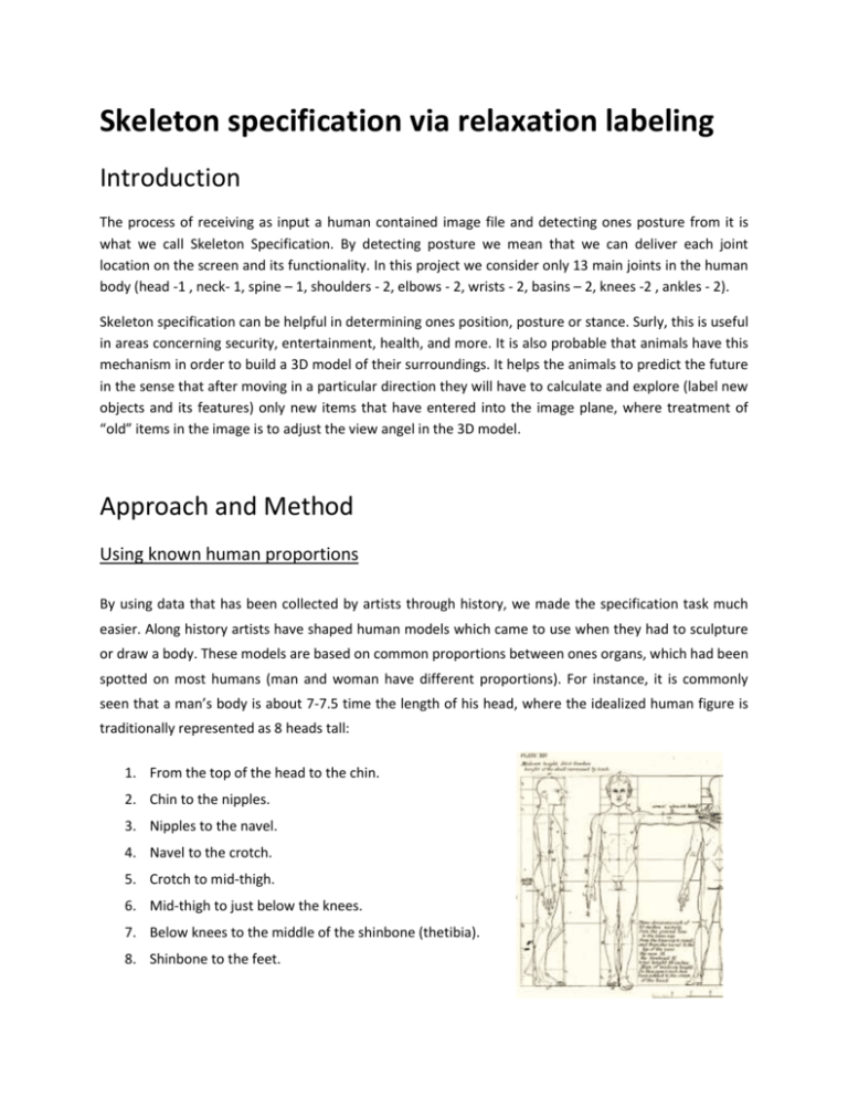
By using data that has been collected by artists through history, we made the specification task much
easier. Along history artists have shaped human models which came to use when they had to sculpture
or draw a body. These models are based on common proportions between ones organs, which had been
spotted on most humans (man and woman have different proportions). For instance, it is commonly
seen that a man’s body is about 7-7.5 time the length of his head, where the idealized human figure is
traditionally represented as 8 heads tall:
1. From the top of the head to the chin.
2. Chin to the nipples.
3. Nipples to the navel.
4. Navel to the crotch.
5. Crotch to mid-thigh.
6. Mid-thigh to just below the knees.
7. Below knees to the middle of the shinbone (thetibia).
8. Shinbone to the feet.
The algorithm
One of the ways the Joints Specification task can be addressed is by splitting the task into two main
stages:
1. Finding N points in the image which are probable to contain joints.
2. Applying the relaxation labeling process on the N2 edges induced by the points in stage 1.
As stage 1 can be assembled from functions available in the openCV library, we decided to tackle the
second stage, and to make it robust against noisy input.
An assumption that must be made for an algorithm that does not hold a stock of human figures is that
its input will be a human figure image on a blank background.
Thus, the input of the algorithm (stage 2) is N points in the plain and a starting edge.
Relaxation labeling
A brief reminder:
Objects = {b1, b2, …, bN} – is the set of objects to be labeled.
Labels = {1, 2, …, m} – is the set of all possible labels.
Pi0 (α) - the measure of confidence that bi should be labeled α.
Rij(α,β) – the strength of compatibility between the hypotheses “bi has label α” and “bj has label
β”.
In our case – the Objects set are the N2 edges, the Labels set is {head, neck, shoulder, elbow, wrist,
spine, knee, ankle} .
Compatibility function Basic compatibility function which had been in use when testing on 4 vertex graph:
1. Comp(e1, e2, A, B) returns the value COMPATIBLE if e1 starts form where e2 ends and A starts
from where B ends.
2. Comp(e1, e2, A, B) returns the value INCOMPATIBLE if e1 and e2 has the same source or
destination.
3. Comp(e1, e2, A, B) returns the value UNKNOWN if the intersection between e1 and e2 is empty.
Improvement #1: Delete “edges” of length 0.
Improvement #2: Delete edges of length bigger then maximum possible label.
Improvement #3: Disqualify edges that contradict limitations induced by human skeleton (for instance:
left thigh can’t have common joint with right arm – this improvement led us to pattern matching).
General graph compatibility function:
The use of pattern matching is in the general graph compatibility function. A human skeleton can be
partially described as a sub graph of the complete graph on 13 vertexes. The new compatibility function
requires entering the wanted sub graph in the form of a list of edges (each built of points from
{1,… , N}). For example EDGES = [(0, 1), (1, 2), (1, 3), (2, 4),(3, 5), (4, 6), (5, 7), (1, 8), (8, 9), (8, 10), (9, 11),
(10, 12), (-1, -1)] is a list describing a man’s skeleton (obviously – undirected one). When activated, as in
comp (e1, e2, A, B) it does pattern matching on the basis of EDGES and return values respectively.
Observation: when examining one route of a directed graph, in each edge, at least one direction is
irrelevant.
After convergence there are two methods of choosing edge labels:
1. For each edge we choose a label that has the greatest probability in the probability vector.
2. For each label we go through all of the probability vectors and find an edge with the maximum
probability for the label (basically we associate a label with an edge that has the greatest
probability for that label) – except the Junk label.
In theory, when convergence happens, the two methods will produce the same result. In reality, it
doesn’t happen. We chose the first method in most tests.
Results
In order to test our method on a simpler model than a man skeleton, we used it on the complete graph
of a square G = (V, E), where V = {(10, 10), (100, 10), (10, 100), (100, 100)}. The Labels are {0, 1, 2, 3, 4},
where 0-3 are the square edges and 4 is an irrelevant edge. The 0 label is automatically given to the
closest edge to the start edge (which is given by the user as input). Here, the compatibility function
encourages two adjacent edges to have two adjacent labels and rejects other possibilities. The initial
graph is in figure 1. The wanted outcome is in figure 2.
(10, 10)
0
3
(10, 100)
(100, 10)
(10, 10)
0
(100, 10)
1
2
Figure 2
(100, 100)
(100, 100)
(10, 100)
Figure 1
The compatibility function being used here is the basic function mentioned above.
Note that the following sustain:


Comp( ((10, 10), (100, 10)), ((100, 10), (100, 100)), 0, 1) > Comp( ((10, 10), (100, 10)),
((100, 100), (100, 10)), 0, 1)
For example, a false labeled square will be as the one in figure 1 after switching
between labels 1 and 3.
Also, say that the start edge given by the user is closest to the edge ((10, 10), (100, 10)), then this edge
automatically gets the label 0.
From this point forward, there are only two possible routes that meet the conditions defined by Comp().
These are:
1. The route you see in figure 2.
2. 0 ((10, 10), (100, 10))
1 ((100, 10), (10, 100))
2 ((10, 100), (100, 100))
3 ((100, 100), (10, 10))
Option 2 creates a “Z” shape route.
Note that the second route does not contradict any of the compatibility function restrictions.
(as seen here – in the HTML file we link
here the right picture) the program finds. The code is in the folder src – converging square.
These are exactly the two routes
Results on a man skeleton
Partial
Figure 3
Figure 4
success.
A green line is a line the algorithm decided of having a relative high chance of being a real edge. The
width of the edge is in direct relationship with its probability of being that edge.
We can see that in the upper body, the only edge that was label correctly is the right forearm, and in the
lower body, the right thigh and the right shin. The algorithm is most “sure” in the edge that starts from
the right shoulder and ends in the right wrist. This is probably because this edge relation to the head is
in the right range.
After running some improvements we got the next outcome.
Figure 5
One can see here, that there are 4 “good” edges, and 2 “bad”. The neck is well noticed, left
shoulder, right arm, and left shin (highest probability). Falsely identified are two edges. One
starts from left wrist to right basin, and second from left wrist to left knee.
Figure 4 and figure 5 present outcome of an algorithm tailored for the human body graph. Next,
we built a versatile algorithm, which is based on pattern matching, rejecting edges that
contradicts human skeleton limitations. Thus, making it hard to wrist-knee edges to appear. This
is the final algorithm we’ve worked on, and its outcome is presented next.
Figure 6
The above is the result of 300 iterations. Each color represents a certain label:
Neck – white, shoulders – red, arms – green, forearms – yellow, spine – pink, thighs- blue, shins –
turquoise, junk - dark gray.
As the 300 iteration is different from the 350 iteration, we don’t have a good estimation about when
we’ll start getting stable result, and good ones. Nevertheless, it seems like the trend is toward a skeleton
which answers the human body limitations. For example, as iterations increases we see less “spines”. A
good thing to notice is that in most edges, both directions of the edge have the same label – this is great
as a skeleton is actually an undirected graph.
Problems
1. Time – a test run on a 4 vertex graph takes a few seconds where a 13 vertex graph run takes 1 to
6 hours.
2. Certain positions make it impossible to detect the right edges by connectivity and distance
measurements alone. For example, a position where basin to shoulder in length is exactly the
length from shoulder to elbow.
Conclusions
1. The method is slow, but given the time, it seems like it will converge to one of the sub-graph
that satisfies the compatibility function conditions.
2. There are probably more efficient ways of getting the right sub-graph.
References
[1] Stephan E. Palmer, "Vision Science – Photons to phenomenology", 1999
[2] http://www.cs.bgu.ac.il/~ben-shahar/Teaching/Computational-Vision//index.php