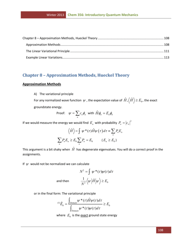
Chem 356: Introductory Quantum Mechanics
Winter 2013
Chapter 8 – Approximation Methods, Hueckel Theory ............................................................................ 108
Approximation Methods ....................................................................................................................... 108
The Linear Variational Principle ............................................................................................................ 111
Example Linear Variations..................................................................................................................... 113
Chapter 8 – Approximation Methods, Hueckel Theory
Approximation Methods
A) The variational principle
For any normalized wave function  , the expectation value of Hˆ , Hˆ  E0 , the exact
groundstate energy.
Proof:  
c 
n n
with Hˆ n  Enn
n
If we would measure the energy we would find En with probability Pn  cn
2
Hˆ    *( ) Hˆ   d   Pn En
n
P E
n
 E0  Pn  E0
n
n
( En  E0 )
n
This argument is a bit shaky when Ĥ has degenerate eigenvalues. You will do a correct proof in the
assignments.
If  would not be normalized we can calculate
N 2    * ( ) ( )d
1
 Ĥ   E0
N2
and then
or in the final form: The variational principle
(1)
E0


 * ( ) Hˆ  ( )d
Domain

 * ( ) ( )d
 E0
Domain
where E0 is the exact ground state energy
108
Chem 356: Introductory Quantum Mechanics
Winter 2013
The variational energy E0 , is exact when  ( )  0 ( ) , the exact ground state wavefunction.
Examples: use a trial wavefunction that depends on one or more parameters  ,  … Then minimize the
trial energy E  ,  
Some simple (trivial) examples:
 1 d2 1 2 
Hˆ h.u    
 x 
2
 2 dx 2 
Take trial wavefunction of the type
 ( x)  e x /2
2
Ne x
Or
2
/2
 ? What is E0 ?
Q:
what is
A:
The exact wavefunction has the form Ne x
Q:
1

2
1
 by minimizing the energy we should get   1 , E0  
2
Take the Hamiltonian for the Hydrogen atom, and an l  0 state
Hˆ 
2
/2
, E0 
d  2 d 
e2
r

2 r 2 dr  dr  4 0 r
2
Take the trial wavefunction e  r
-
What are the integrals to evaluate?
What is the optimal value for  ?
-
What is the value for E0 ?

A:
E0 ( ) 
ˆ  r dr
4  r 2 e r He
0

4  r 2 e r e r dr
0
Minimizing  :
  opt 
1
a0
E0 ( )
0

E0  E0  
1 e2
2 4 0 a0
again: exact a0 
4 0
me2
2
You can do those problems yourself and see if you get the correct answer
Nontrivial example:
Take the Hamiltonian for H-atom, s-orbital, and use the trial wavefunction e r
2
Chapter 8 – Approximation Methods, Hueckel Theory
109
Winter 2013

Chem 356: Introductory Quantum Mechanics
E0 ( ) 

2
ˆ  r 2 dr
4  r 2 e r He
0

4  r 2 e r e r dr
2
2
 ...
0
1
3 2
2e2 2


2me  0 (2 )3/2

E0 3 2
e2


0
 2me (2 )3/2  0 1/2
1
2 
 opt
2me e 2
3(2 )3/2  0
me 2 e4

18 3 0 2
4
E0 ( opt )  
3
E0  
4
 me e4

2
 16  0
E0 ( opt )  0.424
2
2



e2
4 0 a0
1 e2
2 4 0 a0
E0  E0 now, since the trial wavefunction cannot be exact for any 
Note: Gaussian trial orbitals (basis sets) are widely used in electronic structure programs. This is because
integrals are easily evaluated over Gaussians.
This is the origin of the name for the Gaussian Program: It uses Gaussian basic functions!
Chapter 8 – Approximation Methods, Hueckel Theory
110
Winter 2013
Chem 356: Introductory Quantum Mechanics
The Linear Variational Principle
Consider a trial wave function
 ( )   cn f n ( )
n
Let us assume for simplicity
-
Real coefficients, functions, f n  
-
Orthonormal expansion functions:

Domain
f n *( ) f m ( )d   nm
Then we can try to optimize the coefficients
E (c ) 
0
  * ( ) H ( )d
  * ( ) ( )d

N
D
N   cn f n ( ) Hcm f m ( )d
ˆ ( )d
  cn cm  f n ( ) Hf
m
n,m
  cn H nm cm
n,m
D    cn f n ( )cm f m ( )d
n,m
  cn cm  f n ( ) f m ( )d
n,m
  cn cm n ,m   cn 2
n ,m
Then
n
E
 0 k
ck

N
D
DN
ck
  N  ck
0
 
2
ck  D 
D
Or
N  N  D
  
ck  D  ck
N
D
E
ck
ck
N
  H km cm   cn H nk
ck
m
n
D


ck ck
c
n
2
 2ck
n
Chapter 8 – Approximation Methods, Hueckel Theory
111
Winter 2013
Chem 356: Introductory Quantum Mechanics

 

  H km cm  Eck     cn H nk  Eck   0
 m
  n

Since H nk  H kn , this is twice the same equation.

H

c  Eck  0
km m
This has the form of a matrix eigenvalue equation!
m

H  k 





H km
H
and




   
c   c  E
   
   
    
H
c  ck E
km m
m
We can also write
H  E km   c   0
This has the form of a linear equation.
Ac  0 , with A  H  E1
This type of equation only has a solution which det  A  0 .
Hence det  H  E1  0  equation for E “secular determinant”
Let us discuss examples later. For now I want to draw the analogy:
Schrodinger equation Ĥ  E
If we make a basis expansion
   cn f n
f n | f m   nm
n
Then we get a matrix type Schrodinger equation
Hc  Ec
With H  H nm 

n
*( ) Hˆ m ( )d
Such an eigenvalue equation has M solutions for an M  M matrix. They represent approximations
to the ground and excited states.
If the basis is not orthonormal the define Snm 
Or

n
* ( ) Hm ( )d and Hc  ScE (see MQ)
det H  SE  0  eigenvalues E .
Chapter 8 – Approximation Methods, Hueckel Theory
112
Winter 2013
Chem 356: Introductory Quantum Mechanics
Example Linear Variations
Consider particle in the box
 2 d2
H
2m dx 2
2
 n x 
sin 

n
 a 
n ( x) 
Now add to H a linear potential
Use as a trial wave function c1
i, j  1, 2
V0
x
a
2
x
2
2 x
sin
 c2
sin
a
a
a
a
2
2
i x 
d 2 V0
H ij   sin


a
a  2m dx 2 a
V0
16V0 

 E1  2  9 2 


V0 
 16V0
  2 E2  
2
 9
n2 2 2
En 
2ma 2
0 
 0
1
 
2
H

2
16

2mn 
0
  9 2
2
2
2
The eigenvalues of this Hamiltonian are
2
2ma 2
2ma 2
2
16 
 20 
9

0 
4 
2
2

j x
x  sin
a

V0
n
V0
5  0 3
2

 
V
2
2
4 0
2
This happens to be pretty good solution, especially as V0 is small
1/2
2
5  0 1   320  
n 
 9  

2
2   9 2  
1
Chapter 8 – Approximation Methods, Hueckel Theory
113
Winter 2013
Chem 356: Introductory Quantum Mechanics
Other instructive example: consider particle on the ring
2
, with the degenerate m  1 solutions

2mR 2  2
1
cos 
2

E1 
1
2mR 2
sin 


e
Now apply a magnetic field, which adds 
Be Lˆz   Lˆz to the Hamiltonian Lˆz  i
2me

2
Under the influence of the perturbation the levels split. Calculate the energy splitting.
 I used wrong formula; sign is wrong
 
e
2me
  c1
H  H 0   Lz
1

cos   c2
1

sin 
 1

1
 z Lˆz 
cos     i
sin 

 

 1

1
 Lˆz 
sin     i
cos 

 

 2

E
i


2
2mR


H

E
1

= 
 2

 E 
 i

2
 2mR


2
 2

2
det  H  EZ   

E
 
2
 2mR

2
0
 2

 E   

2
 2mR

E 
2
2mR 2

Chapter 8 – Approximation Methods, Hueckel Theory
114
Winter 2013
Chem 356: Introductory Quantum Mechanics
Can I find eigenfunctions?
 2

2
 2mR

 i


  1  2
  1
   


 
2
2
  i   2mR
i 
2 
2mR 
 2

2
 2mR

 i


 1   2
 1 
   


 
2
2
  i   2mR
  i 
2 
2mR 
i
i
What are the eigenfunctions then?
 1
i
   cos   i sin  ~ e
i
1
 i
   cos   i sin  ~ e

i
 
(we normalize,
1
factor)
2
2

 2

2
  i
 i
e 
   ei


2
2
2
 
 2mR 
 2mR

2

 2

2
  i


i

e

   ei



2
2
2
 
 2mR 
 2mR

Bottom line: We can indicate perturbation H  H 0  V
Diagonalize H over degenerate states.
Examples:

( ne )
H-atom: H  H 0  g (v) L  S

Diagonalize Ĥ over 2p orbitals  … 2 p 3 , 2 p 1 eigenfunctions from diagonalizing 6  6
2
2
Hamiltonian. Everything comes out by brute force.
Example 2:
add in additional magnetic interaction
H  H 0 ( ne )  g (v) L  S 
e
2e
Bz Lz 
Bz Sˆz
2me
2me
 diagonalize H over 2p and 2s orbitals
 all the splitting from diagonalization
The linear variational principle is a very powerful tool to calculate approximate eigenfunctions
Chapter 8 – Approximation Methods, Hueckel Theory
115
Winter 2013
Chem 356: Introductory Quantum Mechanics
It is widely used to calculate the splitting of energies in a degenerate manifold, when adding a
perturbation.
When the energies of a Hamiltonian H 0 are not degenerate, one can get a good estimate of the energy
correction due to a perturbation V , by calculating V .
Hence if H 0n  En (0)n , then eigenvalues of Hˆ  Hˆ e  Vˆ are given to first approximation by
n Hˆ n   n * ( )  H 0  V n ( )d
 En (0)   n * ( )V n ( )d
These are just the diagonal elements of the Hamiltonian matrix = First order Perturbation Theory:
 If we go back to box + linear field
H 
2
V
d2
 0x
2
2m dx
a
Ĥ 0
v̂
2 2
2
n x

sin
En (0) 
a
a
2ma 2
V 2 a  n x 
n Vˆ n  0  sin 
 xdx
a a 0
 a 
n 
V0 2  a  V0
   
a a 2 a
V
V
 0 all energies are shifted by 0
a
a


En  En (0)
If zero-order states are degenerate, first-order perturbation theory is useless. Instead use linear
variational principle
Example Lˆ z in sin(mx) basis


choose other basis:  results e im e  im
always diagonalize over zeroth-order states: degenerate first-order perturbation theory
Another example of Hc  cE : Hückel
 -electron theory
In organic chemistry, many molecules are essentially planar. The plane contains “ sp 2 ” carbon, oxygen,
nitrogen atoms. The out of plane Pz -orbitals constitute the
 -orbitals. The molecule’s  - orbitals are
Chapter 8 – Approximation Methods, Hueckel Theory
116
Winter 2013
Chem 356: Introductory Quantum Mechanics
linear combinations of the atomic Pz -orbitals. One can parameterize a one-electron effective
Hamiltonian matrix as follows. Let us restrict ourselves to sp 2 carbons.
  
H 

  
  0 0 

   0 
H 
0   


0 0  
    

  0 0 

H
 0  0 


 0 0  
  0  

   0 

H
0   


 0   
D
Rule:  on diagonal  for any two adjacent atoms connected by a  -bond
  0 ~  Pz (1)V Ne Pz (2) d
Following the variational principle we
a) Diagonalize the Hamiltonian  orbital energies Ek , eigenvectors ck
b) Fill up orbital levels from the bottom up putting an
 and a  electron in each level.
Occupy as many levels as you have  -electrons
c) If levels are degenerate, fill them up with  -electrons first, then add additional  electrons
d) Total energy:

E

occupied
orbitals
e) Density Matrix
Dkl 

 , occupied
ck  cl
E   H kl Dkl (see McQuarrie)
kl
Chapter 8 – Approximation Methods, Hueckel Theory
117
Winter 2013
Chem 356: Introductory Quantum Mechanics
This procedure would work fine in MathCad
How do we do it on paper? Take det  H  E1
 E

0

 E
 ethylene
  E 
 2  0
2
  E   
E  
2 - electrons
Using  and  is a bit tedious for larger problems
 divide each column by  and define x 
 E

 E  x
x 1
 x2  1  0
1 x
E  
x  1
Or
x 1 1
1 x 1 0
1 1 x
x 1 1
1 x 1
x3  1  1  x  x  x  x3  3x  2  0
x 1
1 3  2  0
x  2
8  6  2  0
x
Always:
i
0
 TrN
i
x  1 is double solution.
 x  1  x  2   x2  2x  1  x  2
2
 x3  3x  2
ok
Chapter 8 – Approximation Methods, Hueckel Theory
118
Winter 2013
Chem 356: Introductory Quantum Mechanics
Ek     xk
3  -electrons (4-fold degenerate)
Triplet (3-fold degenerate)
Singlet
What if we would look at the singlet state of the anion?
This is not a stable structure, the molecule would distort
Jahn-Teller Distortion!
I might ask questions of 4 * 4 determinant  too hard to solve
Chapter 8 – Approximation Methods, Hueckel Theory
119
Winter 2013
Chem 356: Introductory Quantum Mechanics
 I would give you the solution x1 , x2 , x3 , x4
You show that ( x  x1 )( x  x2 )( x  x3 )( x  x4 ) is your secular determinant
You can guess the orbitals (phases) from symmetry arguments: The orbitals are always
symmetric or antisymmetric with respect to plane or axis of symmetry
If you know value of x you can solve
x 1 :
 x 1 1  a 

 
 1 x 1  b   0
 1 1 x  c 

 
abc  0
(1 -1 0)
1
1 -2 
orthogonal combinations
x  2 :
 2 1 1 1  0 

   
 1 2 1 1   0 
 1 1 2 1  0 

   
Chapter 8 – Approximation Methods, Hueckel Theory
120