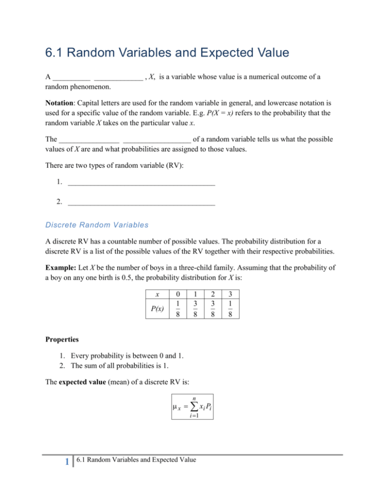
6.1 Random Variables and Expected Value
A __________ _____________ , X, is a variable whose value is a numerical outcome of a
random phenomenon.
Notation: Capital letters are used for the random variable in general, and lowercase notation is
used for a specific value of the random variable. E.g. P(X = x) refers to the probability that the
random variable X takes on the particular value x.
The ________________ __________________ of a random variable tells us what the possible
values of X are and what probabilities are assigned to those values.
There are two types of random variable (RV):
1. _______________________________________
2. _______________________________________
Discrete Random Variables
A discrete RV has a countable number of possible values. The probability distribution for a
discrete RV is a list of the possible values of the RV together with their respective probabilities.
Example: Let X be the number of boys in a three-child family. Assuming that the probability of
a boy on any one birth is 0.5, the probability distribution for X is:
x
P(x)
0
1
8
1
3
8
2
3
8
Properties
1. Every probability is between 0 and 1.
2. The sum of all probabilities is 1.
The expected value (mean) of a discrete RV is:
n
 x   xi Pi
i 1
1
6.1 Random Variables and Expected Value
3
1
8
The variance of a discrete RV is:
n
 2x   ( xi   x )2 Pi
i 1
The standard deviation of a discrete RV is:
 x   2x 
n
 ( xi   x )2 Pi
i 1
Example: In the example above find the following:
1. P( X  2 )
2.  x
3.  x
A probability histogram of a discrete RV is a way to picture the probability distribution.
2
6.1 Random Variables and Expected Value
Continuous Random Variables
A continuous RV takes all the values in an interval of numbers.
Properties
1. The probability distribution of X is described as a density curve (a function always on
or above the x-axis that has area exactly 1 between it and the horizontal axis).
2. The probability of any event is the area under the density curve. The probability of any
individual event is 0.
3. The distinction between  and  is ignored when finding probabilities for continuous RV.
i.e. P(a < X < b) = P(a £ X £ b) = P(a < X £ b) = P(a £ X < b) .
The normal distribution is an example of a probability distribution and the normal curve is a
density curve.
Worksheet: “Transforning and Combining Random Variables”
Transforming Random Variables
The random variable X can be transformed by adding a constant to each value, or by multiplying each
value by a constant, or some linear combination of the two. The rules for the mean, variance and standard
deviation of the new transformed random variable are:
a bX  a  b X
 a2bX  b 2 X2
 a bX  b  X
Notice the similarity to the rules for the statistics of one variable data (remember “rescaling and
recentering”?).
3
6.1 Random Variables and Expected Value
Combining Random Variables
Sometimes you may also wish to combine two different random variables. The rules for the mean,
variance and standard deviation of the combined random variables are not so straightforward:
mean m X +Y = m X + mY
m X -Y = m X - mY
variance s 2X +Y = s 2X + s Y2 if and only if X and Y are independent
s 2X -Y = s 2X + s Y2 if and only if X and Y are independent
standard deviation s X +Y = s 2X + s Y2 if and only if X and Y are independent
s X -Y = s 2X + s Y2 if and only if X and Y are independent
Notice how you only ever add variances, even if the two random variables are subtracted. NEVER ADD
STANDARD DEVIATIONS.
Example 1: Consider a distribution with
X 14,  X  2. Multiply each value of X by 4, and then add
3 to each. Find the mean and standard deviation of the transformed random variable.
s 3+4 X =
m3+4 X =
Example 2: X is the number of cars that Linda sells.
Cars Sold (X)
Probability
0
0.3
1
0.4
2
0.2
3
0.1
Y is the number of trucks and SUVs that Linda sells.
Trucks & SUVs Sold (Y)
Probability
0
0.4
1
0.5
2
0.1
mY =
mX =
At her commission rate of 25% of gross profit on each vehicle she sells, Linda expects to earn $350 for
each car sold and $400 for each truck or SUV sold. So her earnings, Z, are:
Z = __________________________________
Linda’s mean earnings are:
mZ =
4
6.1 Random Variables and Expected Value