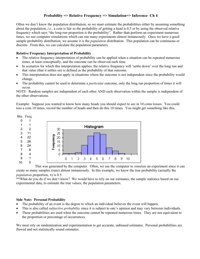
Probability => Relative Frequency => Simulation=> Inference Ch 4
Often we don’t know the population distribution, so we must estimate the probabilities either by assuming something
about the population, i.e., a coin is fair so the probability of getting a head is 0.5 or by using the observed relative
frequency which says “the long-run proportion is the probability”. Rather than perform an experiment numerous
times, we use computer simulations which can run many experiments almost instaneously. Once we have a good
sample probability distribution, we assume it is the population distribution. This population can be continuous or
discrete. From this, we can calculate the population parameters.
Relative Frequency Interpretation of Probability
 The relative frequency interpretation of probability can be applied when a situation can be repeated numerous
times, at least conceptually, and the outcome can be observed each time.
 In scenarios for which this interpretation applies, the relative frequency will ‘settle down’ over the long run and
that value (that it settles on) is defined as the probability of that outcome.
 This interpretation does not apply in situations where the outcome is not independent since the probability would
change.
 The probability cannot be used to determine a particular outcome, only the long run proportion of times it will
occur.
NOTE: Random samples are independent of each other AND each observation within the sample is independent of
the other observations.
Example: Suppose you wanted to know how many heads you should expect to see in 10 coins tosses. You could
toss a coin 10 times, record the number of heads and then do this 10 times. You might get something like this.
Bin Freq
0
1
2
3
4
5
6
7
8
9
10
1
1
2
11
22
26
24
8
4
1
0
This was generated by the computer. Often, we use the computer to simulate an experiment since it can
create so many samples (runs) almost instaneously. In this example, we know the true probability (actually the
population proportion, ) is 0.5.
**What do you do if we don’t know? We would have to rely on our estimates, the sample statistics based on our
experimental data, to estimate the true values, the population parameters.
Side Note: Personal Probability
 The probability of an event is the degree to which an individual believes the event will happen.
 This is also called subjective probability since it is subject to one’s opinion and may vary between individuals.
 These probabilities are used when the outcome cannot be repeated numerous times. They are not equivalent to
the proportion or percentage of occurrences.
We must rely on randomization and experimentation to get accurate, unbiased estimates. Personal probabilities are
flawed and not statistically sound estimates.
Random Variables --- Ch 4.3
A random variable assigns a number to each outcome of a random circumstance. A discrete random variable can
only take one of a countable number of distinct values. The probabilties for each value along with the actual values
make up the population distribution of the random variable, and we can represent this in a table or relative frequency
histogram.
Mean of a Discrete Population, X = Xp(X) = E(X), the expected value of X
The sum of each of the values of X times the probability it occurred equals the mean. Since this is the entire
distribution, not just a sample, this mean is (X).
Variance of a Discrete Population, X2 = (X - )2p(X)
To find the variance (remember, we must always find the variance to get the standard deviation), 2(X), we subtract
the mean from each observation, square that difference and multiply by the probability of that observation occurring.
Then we sum all of these to get 2(X). The standard deviation, (X), is just the positive square root of the variance.
Rules for Means:
Let X and Y be two random variables, and a,b,c be constants (i.e., any number)
1. a = E(a) = a
2. aX = E(aX) = aX
3. a  X = E(a  X) = a  X
In general, aX  bY  c = E(aX  bY  c) = aX  bY  c
Note: think of a and b as scales changes and c as a shift change!
and Variances:
1. 2a = V(a) = 0
2. 2aX = V(aX) = a22X
3. 2a  X = V(a  X) = 2X
In general, if X and Y are INDEPENDENT, 2aX  bY  c = V(aX  bY  c) = a22X + b22Y and
aX  bY  c = (aX  bY  c) = (a22X + b22Y)  aX + bY !!!!!!!!
Continuous random variables cannot be displayed in a table since there are innumerable values. These are
displayed as curves, and probabilities are proportions of these curves (areas under the curve) so you need calculus
when it’s not easy to find the area. Fortunately, we have tables that have already done this for us. In general, there is
NO area at an exact point, so we find probabilities for ranges of values. So, for any continuous random variable, X,
P(X = a) = 0
P(X  a) = P(X < a)
P(X  b) = P(X > b)
P(a  X  b) = P(X < b) - P(X < a)
One of the most common continuous random variables is the normal, that familiar bell-shaped curve. There are 2
parameters that totally define a normal curve: the mean, , which is the center (and peak), and the variance, which
defines the spread. The Standard Normal is the most basic of the normal curves with mean, =0 and standard
deviation, =1. We will use the notation: Z ~ N(0, 12), where the 1st number is the mean and 2nd is the variance. I
will always use the variance equal to the standard deviation squared within the parentheses.
The Z Table gives you probabilities for the standard normal. The probabilities, are listed in the body of the table and
are the areas to the left of the z*s which are the row and column headings, the column being the hundredth digit for
the row z*. To find areas to the right, remember that the Standard Normal is symmetric about 0, so just convert the
sign of the z*: P(Z  z*)=P(Z-z*).
We can convert any nonstandard normal X ~ N(x, x2) to a standard normal by: z = ( x - x)/x. So, if
X ~ N( x, 2x), then z = (x - x)/x ~ N( 0, 1).
We can also create (or convert backwards) any nonstandard normals by: x = x + z*x.