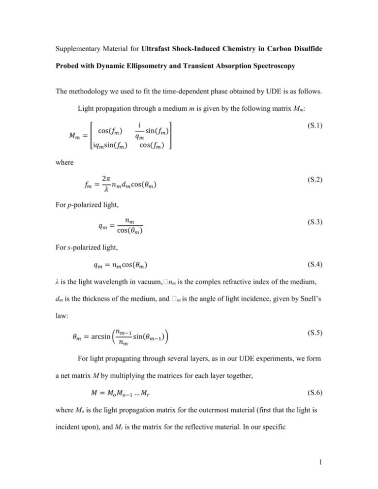
Supplementary Material for Ultrafast Shock-Induced Chemistry in Carbon Disulfide
Probed with Dynamic Ellipsometry and Transient Absorption Spectroscopy
The methodology we used to fit the time-dependent phase obtained by UDE is as follows.
Light propagation through a medium m is given by the following matrix Mm:
𝑀𝑚 = [
cos⁡(𝑓𝑚 )
i𝑞𝑚 sin⁡(𝑓𝑚 )
i
sin⁡(𝑓𝑚 )
]
𝑞𝑚
cos⁡(𝑓𝑚 )
(S.1)
where
𝑓𝑚 =
2𝜋
𝑛 𝑑 cos⁡(𝜃𝑚 )
𝜆 𝑚 𝑚
(S.2)
For p-polarized light,
𝑞𝑚 =
𝑛𝑚
cos⁡(𝜃𝑚 )
(S.3)
For s-polarized light,
𝑞𝑚 = 𝑛𝑚 cos⁡(𝜃𝑚 )
(S.4)
λ is the light wavelength in vacuum,�nm is the complex refractive index of the medium,
dm is the thickness of the medium, and �m is the angle of light incidence, given by Snell’s
law:
𝑛𝑚−1
𝜃𝑚 = arcsin⁡(
sin(𝜃𝑚−1 ))
𝑛𝑚
(S.5)
For light propagating through several layers, as in our UDE experiments, we form
a net matrix M by multiplying the matrices for each layer together,
𝑀 = 𝑀𝑜 𝑀𝑜−1 … 𝑀𝑟
(S.6)
where Mo is the light propagation matrix for the outermost material (first that the light is
incident upon), and Mr is the matrix for the reflective material. In our specific
1
experiments, the order of materials from outermost to reflective are as follows: CaF2,
unshocked liquid, shocked liquid, 5 nm Al2O3, and the aluminum drive layer. The only
variables in M that change with time in our shock experiments are the thicknesses of the
unshocked and shocked liquid layers. For a constant velocity shock, the thickness of the
unshocked layer with time, du(t), is
𝑑u (𝑡) = 𝑑0 − 𝑢s 𝑡
(S.7)
where us is the shock velocity and d0 is the initial thickness of the unshocked layer. The
thickness of the shocked layer, ds(t) can be described as
𝑑𝑠 (𝑡) = (𝑢𝑠 − 𝑢𝑝 )𝑡
(S.8)
where up is the particle velocity of the Al/liquid interface. Thus, our matrix M is timedependent, with the variables us, up, and ns (refractive index of the shocked liquid layer)
to be solved for. Since equations S.1 – S.6 are independent of shock dynamics, any
number of layers or material dynamics can be included in the same framework. We
include a shock risetime to accelerate the wave continuously from zero to the final
velocity to better match the shock experiments.
The total reflection amplitude for p- and s-polarized light are defined as Rp and Rs,
respectively, and are given generally as
𝑅=
𝑀1,1 𝑞𝑜 − 𝑀2,2 𝑞𝑟 + 𝑀1,2 𝑞𝑜 𝑞𝑟 − 𝑀2,1
= 𝜌𝑒 𝑖𝜙
𝑀1,1 𝑞𝑜 + 𝑀2,2 𝑞𝑟 − 𝑀1,2 𝑞𝑜 𝑞𝑟 + 𝑀2,1
(S.9)
where, as above, the subscript ‘o’ refers to the outermost layer and ‘r’ refers to the
reflective layer. The subscripts of M refer to the matrix elements of the total light
propagation matrix given above; for example, M1,2 is the matrix element at row 1, column
2. The reflectance is determined by the modulus squared of the reflection amplitude,
|R|2 = |ρ|2 and ϕ is the phase of the light upon reflection. By calculating the phase of the
2
shocked material stack at a given time and subtracting the phase from the initial material
stack, experimentally observable phase change dynamics can be calculated.
In practice, we do not measure the absolute phase of the reflected light, but rather
the change in phase caused by the change in layer thickness with time and the motion of
the reflecting surface due to the shock. Likewise, we interrogate the ratio of the reflection
amplitude containing us, up, and ns to that of the initial, unshocked layered sample:
𝑅(𝑡) 𝜌(𝑡) 𝑖Δ𝜙(𝑡)
=
𝑒
𝑅0
𝜌0
(S.10)
∆𝜙(𝑡) = 𝜙(𝑡) − 𝜙0
(S.11)
Where the subscript ‘0’ denotes the unshocked material, where us and up=0 and there is
no term for ns as there is no shocked layer.
Our experiments yielded time-dependent phase shifts for s- and p-polarizations
for both a low angle and high angle interferometer, a total of four sets of data. The values
of up, us, and ns, were adjusted to minimize the difference between the calculated and
observed data sets of optical phase shift as well as the phase derivatives to Eqs. S.1-S.11
using a Levenburg-Marquardt least squares fitting algorithm in LabView (National
Instruments). Input parameters were the unshocked refractive indices for all layers, probe
wavelength, incident probe angle, and an estimate of each layer thickness. An initial
guess at the fit parameters used as input to the Levenburg-Marquardt optimization are
produced by fitting the low angle data over a region of ~100-200 ps, taken significantly
after any shock risetime effects, to the model described in Armstrong, et al.1 The fringe
frequency, depth, and offset are fit to determine the refractive index change and shock
and particle velocity.
3
Table S1: Ultrafast Dynamic Ellipsometry (UDE) data points for carbon disulfide (CS2)
from this study. up: particle velocity, us: shock velocity, ns: shocked refractive index
(real)
up (km/s)
us (km/s)
ns
0.45
2.26
0.45
2.26
0.64
2.34
0.64
2.56
0.73
2.40
0.78
2.68
0.82
2.70
1.00
3.00
1.05
3.17
1.19
3.85
1.20
3.51
1.24
3.96
1.25
3.93
1.25
3.66
1.27
3.63
1.27
3.52
1.29
3.98
1.29
3.60
1.30
3.59
1.33
3.95
1.35
3.91
1.36
3.83
1.36
3.98
1.37
4.04
1.37
4.00
1.37
3.87
1.43
3.91
1.44
3.89
1.48
4.23
1.49
3.92
1.49
4.10
1.50
3.89
1.61
4.02
1.69
4.01
1.80
4.12
1.79
1.78
1.85
1.85
1.97
1.91
1.94
2.04
2.02
2.00
2.06
2.09
2.08
2.05
2.13
2.12
2.08
2.14
2.14
2.12
2.13
2.13
2.17
2.06
2.17
2.16
2.13
2.17
2.15
2.24
2.24
2.28
2.26
2.41
2.40
4
Table S2: UDE data for CS2 from Bolme2
up
us
0.18
0.18
0.30
0.31
0.31
0.38
0.41
0.42
0.42
0.46
0.46
0.47
0.49
0.50
0.51
0.51
0.53
0.56
0.57
0.57
0.59
0.59
0.64
0.93
1.20
1.83
1.83
1.90
1.92
1.95
2.07
2.10
2.13
2.20
2.27
2.30
2.44
2.46
2.46
2.54
2.56
ns
1.71
1.71
1.88
1.94
1.93
2.01
2.05
2.09
1.93
2.10
2.06
2.26
2.28
2.08
2.29
2.16
2.28
2.35
2.34
2.24
2.39
2.23
2.24
2.90
2.94
3.79
3.79
3.81
4.04
3.81
4.09
3.92
4.12
4.14
4.01
4.06
4.45
4.50
4.49
4.51
4.57
1.69
1.69
1.74
1.79
1.77
1.77
1.81
1.87
1.80
1.83
1.83
1.78
1.78
1.84
1.80
1.83
1.81
1.83
1.84
1.85
1.85
1.87
1.90
2.18
2.40
2.62
2.62
2.68
2.77
2.74
2.86
2.87
2.91
2.98
3.05
3.07
3.04
3.08
3.15
3.28
3.24
5
Table S3: Impedance-matched data points for CS2 from this study. σ: one standard
deviation
up (km/s)
up σ (km/s) us (km/s)
us σ (km/s)
1.99
0.10
4.00
0.06
2.14
0.09
3.71
0.07
2.17
0.06
4.14
0.13
2.37
0.12
4.44
0.22
2.40
0.11
4.09
0.14
2.47
0.07
4.06
0.12
2.51
0.08
3.96
0.23
2.54
0.08
4.00
0.10
2.56
0.05
4.03
0.08
2.78
0.10
4.80
0.21
2.78
0.09
4.71
0.08
2.97
0.14
4.98
0.14
2.98
0.19
4.91
0.35
3.02
0.19
5.24
0.31
3.18
0.17
5.25
0.07
3.22
0.12
5.20
0.28
3.36
0.33
5.45
0.27
3.37
0.18
5.49
0.63
3.39
0.21
5.48
0.18
1
2
M. R. Armstrong, J. C. Crowhurst, S. Bastea, and J. M. Zaug, J. Appl. Phys. 108,
023511 (2010).
C. A. Bolme, Ph. D. thesis, Massachusetts Institute of Technology, 2008.
6