Lesson 10
NYS COMMON CORE MATHEMATICS CURRICULUM
M4
ALGEBRA II
Lesson 10: Normal Distributions
Student Outcomes

Students calculate 𝑧 scores.

Students use technology and tables to estimate the area under a normal curve.

Students interpret probabilities in context.
Lesson Notes
In this lesson, students calculate 𝑧 scores and use technology and tables to estimate the area under a normal curve.
Depending on technology resources available to students, teachers may need to have students work with a partner or in
small groups.
Classwork
Exercise 1 (3 minutes)
This first exercise is a review of what is meant by a normal distribution. Use this as an opportunity to informally assess
students’ understanding of different distribution types by having students attempt the exercises independently.
Exercise 1
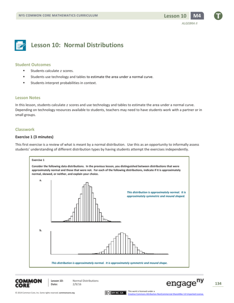
Consider the following data distributions. In the previous lesson, you distinguished between distributions that were
approximately normal and those that were not. For each of the following distributions, indicate if it is approximately
normal, skewed, or neither, and explain your choice.
a.
This distribution is approximately normal. It is
approximately symmetric and mound shaped.
b.
This distribution is approximately normal. It is approximately symmetric and mound shape.
Lesson 10:
Date:
Normal Distributions
2/9/16
© 2014 Common Core, Inc. Some rights reserved. commoncore.org
134
This work is licensed under a
Creative Commons Attribution-NonCommercial-ShareAlike 3.0 Unported License.
Lesson 10
NYS COMMON CORE MATHEMATICS CURRICULUM
M4
ALGEBRA II
c.
This distribution is not symmetric; therefore, it
is not approximately normal. This distribution
is skewed to the right as it has most of the data
values in the beginning and then tapers off. It
has a longer tail on the right.
b.
This distribution is approximately normal. It is symmetric
and mound shaped.
c.
This distribution is not approximately normal. It is
symmetric but not mound shaped. This distribution,
however, is also not skewed. It does not have a longer tail
on one side. It would be described as approximately a
uniform distribution. Note that this distribution was
discussed in earlier grades. It is important to emphasize
that there are other types of data distributions and that
not all are either approximately normal or skewed.
A normal distribution is a distribution that has a particular symmetric mound shape, as shown below.
Lesson 10:
Date:
Normal Distributions
2/9/16
© 2014 Common Core, Inc. Some rights reserved. commoncore.org
135
This work is licensed under a
Creative Commons Attribution-NonCommercial-ShareAlike 3.0 Unported License.
Lesson 10
NYS COMMON CORE MATHEMATICS CURRICULUM
M4
ALGEBRA II
Exercise 2 (5 minutes)
Scaffolding:
This exercise introduces students to 𝑧 scores. Prior to having the students tackle
this exercise (or after they have completed it), it might be helpful to familiarize
them with the reason why 𝑧 scores are important. You could open this discussion
with the following:

MP.3
Suppose that you took a math test and a Spanish test. The mean score
for both tests was 80. You got an 86 in math and a 90 in Spanish. Did
you necessarily do better in Spanish relative to your fellow students?

No. For example, suppose the standard deviation of the math
scores was 4 and the standard deviation of the Spanish scores
1
2
was 8. Then my score of 86 in math is 1 standard deviations
1
4
above the mean, and my score in Spanish is only 1 standard
deviations above the mean. Relative to the other students, I did
better in math.
In the above example, the 𝑧 score for math is 1.5, and the 𝑧 score for Spanish is
1.25. Negative 𝑧 scores indicate values that are below the mean.
Ask students to state in their own words what a 𝑧 score is. Essentially look for an
early understanding that a 𝑧 score measures distance in units of the standard
deviation. For example, a 𝑧 score of 1 represents an observation that is at a
distance of 1 standard deviation above the mean.
Exercise 2
 For students who may be
struggling, consider framing the
question this way, “Suppose that
you took a math test and a Spanish
test. The mean for both tests was
80; the standard deviation of the
math scores was 8. You got an 86
in math and a 90 in Spanish. On
which test did you do better than
most of your classmates?”
Consider showing a visual of sample
data distributions for each to aid
understanding.
 For more advanced learners,
consider posing the question this
way, “Suppose that you took a
math test and a Spanish test. The
mean score for both was 80. You
got an 86 in math and a 90 in
Spanish. On which test did you do
better than most of your
classmates. Explain your
reasoning.”
When calculating probabilities associated with normal distributions, 𝒛 scores are used. A 𝒛 score for a particular value
measures the number of standard deviations away from the mean. A positive 𝒛 score corresponds to a value that is
above the mean, and a negative 𝒛 score corresponds to a value that is below the mean. The letter 𝒛 was used to
represent a variable that has a standard normal distribution where the mean is 𝟎 and standard deviation is 𝟏. This
distribution was used to define a 𝒛 score. A 𝒛 score is calculated by
𝒛=
a.
𝒗𝒂𝒍𝒖𝒆 − 𝒎𝒆𝒂𝒏
.
𝒔𝒕𝒂𝒏𝒅𝒂𝒓𝒅 𝒅𝒆𝒗𝒊𝒂𝒕𝒊𝒐𝒏
The prices of the printers in a store have a mean of $𝟐𝟒𝟎 and a standard deviation of $𝟓𝟎. The printer that you
eventually choose costs $𝟑𝟒𝟎.
i.
What is the 𝒛 score for the price of your printer?
𝒛=
ii.
𝟑𝟒𝟎 − 𝟐𝟒𝟎
=𝟐
𝟓𝟎𝟎
How many standard deviations above the mean was the price of your printer?
My printer was 𝟐 standard deviations above the mean price.
b.
Ashish’s height is 𝟔𝟑 inches. The mean height for boys at his school is 𝟔𝟖. 𝟏 inches, and the standard deviation of
the boys’ heights is 𝟐. 𝟖 inches.
i.
What is the 𝒛 score for Ashish’s height? (Round your answer to the nearest hundredth.)
𝒛=
𝟔𝟑 − 𝟔𝟖. 𝟏
= −𝟏. 𝟖𝟐
𝟐. 𝟖
Lesson 10:
Date:
Normal Distributions
2/9/16
© 2014 Common Core, Inc. Some rights reserved. commoncore.org
136
This work is licensed under a
Creative Commons Attribution-NonCommercial-ShareAlike 3.0 Unported License.
Lesson 10
NYS COMMON CORE MATHEMATICS CURRICULUM
M4
ALGEBRA II
ii.
What is the meaning of this value?
Ashish’s height is 𝟏. 𝟖𝟐 standard deviations below the mean height for boys at his school.
c.
Explain how a 𝒛 score is useful in describing data.
A 𝒛 score is useful in describing how far a particular point is from the mean.
Example 1 (10 minutes): Use of 𝒛 Scores and a Graphing Calculator to find Normal Probabilities
In this example, students are introduced to the process of calculating normal probabilities, and in this example and the
two exercises that follow, 𝑧 scores are used along with a graphing calculator. (The use of tables of normal probabilities is
introduced later in this lesson, and the use of spreadsheets is introduced in the next lesson.) Encourage students to
always draw normal distribution curves and to show their work on the graph when working problems that involve a
normal distribution.
Work through Example 3 with the class showing students how to calculate the relevant 𝑧 scores and use a graphing
calculator* to find the probability of interest. Students new to the curriculum may need additional support with the
graphing calculator.
*Calculator note: The general form of this is Normalcdf([left z bound],[right z bound]). The Normalcdf function is
accessed using 2nd, DISTR. On selecting 2nd DISTR, some students using the more recent TI-84 operating systems might
be presented with a menu asking for left bound, right bound, mean, and standard deviation. This can be avoided by
having these students do the following: press 2nd, QUIT (to return to the home screen); press MODE; scroll down to the
“NEXT” screen; set STAT WIZARDS to OFF.
Example 1: Use of 𝒛 Scores and a Graphing Calculator to find Normal Probabilities
A swimmer named Amy specializes in the 𝟓𝟎 meter backstroke. In competition her mean time for the event is
𝟑𝟗. 𝟕 seconds, and the standard deviation of her times is 𝟐. 𝟑 seconds. Assume that Amy’s times are approximately
normally distributed.
a.
Estimate the probability that Amy’s time is between 𝟑𝟕 and 𝟒𝟒 seconds.
The first time is a little less than 𝟐 standard deviations from her mean time of 𝟑𝟗. 𝟕 seconds. The second time is
nearly 𝟐 standards deviations above her mean time. As a result, the probability of a time between the two values
covers nearly 𝟒 standard deviations and would be rather large. I estimate 𝟎. 𝟗 or 𝟗𝟎%.
b.
Using 𝐳 scores and a graphing calculator and rounding your answers to the nearest thousandth, find the probability
that Amy’s time in her next race is between 𝟑𝟕 and 𝟒𝟒 seconds.
The 𝒛 score for 𝟒𝟒 is
𝟑𝟕−𝟑𝟗.𝟕
𝟐.𝟑
𝟒𝟒−𝟑𝟗.𝟕
= 𝟏. 𝟖𝟕𝟎, and the 𝒛 score for 𝟑𝟕 is
𝟐.𝟑
= −𝟏. 𝟏𝟕𝟒
The probability that Amy’s time is between 𝟑𝟕 and 𝟒𝟒 seconds is then found to be
𝟎. 𝟖𝟒𝟗.
(Note: If students are using TI-83 or TI-84 calculators, this result is found by
entering Normalcdf(−𝟏. 𝟏𝟕𝟒, 𝟏. 𝟖𝟕𝟎).)
Lesson 10:
Date:
Normal Distributions
2/9/16
© 2014 Common Core, Inc. Some rights reserved. commoncore.org
137
This work is licensed under a
Creative Commons Attribution-NonCommercial-ShareAlike 3.0 Unported License.
Lesson 10
NYS COMMON CORE MATHEMATICS CURRICULUM
M4
ALGEBRA II
c.
Estimate the probability that Amy’s time is more than 𝟒𝟓 seconds.
𝟒𝟓 seconds is more than 𝟐 standard deviations from the mean of 𝟑𝟗. 𝟕 seconds. There is a small probability that
her time will be greater than 𝟒𝟓 seconds. I estimate 𝟎. 𝟎𝟑 or 𝟑%.
d.
Using 𝐳 scores and a graphing calculator and rounding your answers to the nearest thousandth, find the probability
that Amy’s time in her next race is more than 𝟒𝟓 seconds.
The 𝒛 score for 𝟒𝟓 is
𝟒𝟓−𝟑𝟗.𝟕
𝟐.𝟑
= 𝟐. 𝟑𝟎𝟒.
The probability that Amy’s time is more than 𝟒𝟓 seconds is then
found to be 𝟎. 𝟎𝟏𝟏.
(Note: This result is found by entering Normalcdf(𝟐. 𝟑𝟎𝟒, 𝟗𝟗𝟗) or
the equivalent of this for other brands of calculator. The keystroke
for positive infinity on some calculators is 1EE99. The number
“𝟗𝟗𝟗” can be replaced by any large positive number. Strictly
speaking, the aim here is to find the area under the normal curve
between 𝒛 = 𝟐. 𝟑𝟎𝟒 and positive infinity. However, it is impossible
to enter positive infinity into the calculator, so any large positive
number can be used in its place.)
d.
What is the probability that Amy’s time would be at least 𝟒𝟓 seconds?
Since Amy’s times have a continuous distribution, the probability of “more than 𝟒𝟓 seconds” and the probability of
“at least 𝟒𝟓 seconds” are the same. So the answer is the same as part (d), 𝟎. 𝟎𝟏𝟏.
(It is worth pointing out to students that this will apply to any question about the normal distribution.)
e.
Using 𝐳 scores and a graphing calculator and rounding your answers to the nearest thousandth, find the probability
that Amy’s time in her next race is less than 𝟑𝟔 seconds.
The 𝒛 score for 𝟑𝟔 is
𝟑𝟔−𝟑𝟗.𝟕
𝟐.𝟑
= −𝟏. 𝟔𝟎𝟗.
The probability that Amy’s time is less than 36 seconds is then found to be
𝟎. 𝟎𝟓𝟒.
(This result is found by entering Normalcdf(−𝟗𝟗𝟗, −𝟏. 𝟔𝟎𝟗) or the
equivalent of this for other brands of calculator. Here “−𝟗𝟗𝟗” is being
used in place of negative infinity; any large negative number can be used
in its place. The keystroke on some calculators for negative infinity is
–1EE99.)
Exercise 3 (8 minutes)
This exercise provides practice with the skills students have learned in Example 2. Again, encourage students to draw a
MP.4 normal distribution curve for each part of the exercise showing work on their graphs in order to answer questions about
the distribution. Let students work independently (if technology resources allow) and confirm answers with a neighbor.
Lesson 10:
Date:
Normal Distributions
2/9/16
© 2014 Common Core, Inc. Some rights reserved. commoncore.org
138
This work is licensed under a
Creative Commons Attribution-NonCommercial-ShareAlike 3.0 Unported License.
Lesson 10
NYS COMMON CORE MATHEMATICS CURRICULUM
M4
ALGEBRA II
Exercise 3
The distribution of lifetimes of a particular brand of car tires has a mean of 𝟓𝟏, 𝟐𝟎𝟎 miles and a standard deviation of
𝟖, 𝟐𝟎𝟎 miles.
a.
Assuming that the distribution of lifetimes is approximately normally distributed and rounding your answers to the
nearest thousandth, find the probability that a randomly selected tire lasts
i.
between 𝟓𝟓, 𝟎𝟎𝟎 and 𝟔𝟓, 𝟎𝟎𝟎 miles.
𝑷(between 𝟓𝟓, 𝟎𝟎𝟎 and 𝟔𝟓, 𝟎𝟎𝟎) = 𝟎. 𝟐𝟕𝟓
ii.
less than 𝟒𝟖, 𝟎𝟎𝟎 miles.
𝑷(< 𝟒𝟖, 𝟎𝟎𝟎) = 𝟎. 𝟑𝟒𝟖
iii.
at least 𝟒𝟏, 𝟎𝟎𝟎 miles.
𝑷(> 𝟒𝟏, 𝟎𝟎𝟎) = 𝟎. 𝟖𝟗𝟑
b.
Explain the meaning of the probability that you found in part (a–iii).
If a large number of tires of this brand were to be randomly selected, then you would expect about 𝟖𝟗. 𝟑% of them
to last more than 𝟒𝟏, 𝟎𝟎𝟎 miles.
Lesson 10:
Date:
Normal Distributions
2/9/16
© 2014 Common Core, Inc. Some rights reserved. commoncore.org
139
This work is licensed under a
Creative Commons Attribution-NonCommercial-ShareAlike 3.0 Unported License.
Lesson 10
NYS COMMON CORE MATHEMATICS CURRICULUM
M4
ALGEBRA II
Exercise 4 (5 minutes)
Here students have to understand the idea of the lifetime of a tire being “within 10,000 miles of the mean.” Some
discussion of this idea might be necessary. Ask students what they think the statement is indicating about the lifetime of
MP.3 a tire. As they share their interpretations, record their summaries. Encourage students to use pictures, possibly
involving a normal distribution, in their explanations. In this exercise, students can practice constructing arguments and
critiquing the reasoning of others based on their understanding of a normal distribution.
Exercise 4
Think again about the brand of tires described in Exercise 3. What is the probability that the lifetime of a randomly
selected tire is within 𝟏𝟎, 𝟎𝟎𝟎 miles of the mean lifetime for tires of this brand?
𝑷(within 𝟏𝟎, 𝟎𝟎𝟎 of mean) = 𝟎. 𝟕𝟕𝟖
Example 2 (7 minutes): Using Table of Standard Normal Curve Areas
The last part of this lesson is devoted to the process of using tables of normal probabilities in place of the “Normalcdf”
(or equivalent) function on the calculator. Completion of this example will enable students who do not have access to a
graphing calculator at home to complete the Problem Set. (However, if time is short, then this example could be
reserved for Lesson 11, in which case Problem Set Question 4 should be omitted from the assignment, and Lesson 11
should begin with this example.) Work through this example as a class showing students how to use the table to
estimate the area under a normal curve.
Example 2: Using Table of Standard Normal Curve Areas
The standard normal distribution is the normal distribution with a mean of 𝟎 and a standard deviation of 𝟏. The diagrams
below show standard normal distribution curves. Use a table of standard normal curve areas to determine the shaded
areas.
a.
The provided table of normal areas gives the area to the left of the
selected 𝒛 score. So, here, you find 𝟏. 𝟐 in the column on the very
left of the table, and then move horizontally to the column headed
“𝟎. 𝟎𝟑.” The table gives the required area (probability) to be
𝟎. 𝟖𝟗𝟎𝟕.
0
Lesson 10:
Date:
z = 1.23
Normal Distributions
2/9/16
© 2014 Common Core, Inc. Some rights reserved. commoncore.org
140
This work is licensed under a
Creative Commons Attribution-NonCommercial-ShareAlike 3.0 Unported License.
Lesson 10
NYS COMMON CORE MATHEMATICS CURRICULUM
M4
ALGEBRA II
b.
In the left-hand column of the table find −𝟏. 𝟖 and move
horizontally to the column labeled 𝟎. 𝟎𝟔. The table gives a
probability of 𝟎. 𝟎𝟑𝟏𝟒. Note that the table always supplies the
area to the left of the chosen 𝒛 score. Also, note that the total
area under any normal curve is 𝟏. (This is the case for any
probability distribution curve.) So, the required area, which is the
area to the right of −𝟏. 𝟖𝟔, is 𝟏 − 𝟎. 𝟎𝟑𝟏𝟒 = 𝟎. 𝟗𝟔𝟖𝟔.
z= -1.86
0
c.
The approach here is to find the area to the left of 𝒛 = 𝟐 and to
subtract the area to the left of 𝒛 = −𝟏. The table gives the area
to the left of 𝒛 = 𝟐. 𝟎𝟎 to be 𝟎. 𝟗𝟕𝟕𝟐 and the area to the left of
𝒛 = −𝟏. 𝟎𝟎 to be 𝟎. 𝟏𝟓𝟖𝟕. So, the required area is
𝟎. 𝟗𝟕𝟕𝟐 − 𝟎. 𝟏𝟓𝟖𝟕 = 𝟎. 𝟖𝟏𝟖𝟓.
z= -1
z=2
0
Closing (2 minutes)
Remind students to be aware of order when calculating 𝑧 scores. Refer back to Exercise 2.

The prices of printers in a store have a mean of $240 and a standard deviation of $50. The printer that you
eventually choose costs $340. What is wrong with the following 𝑧 score? How do you know?
240 − 340 −100
𝑧=
=
= −2
50
50

The 𝑧 score is negative, when it should be positive. The printer I chose is greater than the mean, which
should result in a positive 𝑧 score.
Have students interpret a probability in their own words. For example, refer back to Example 1.

A swimmer named Amy specializes in the 50 meter backstroke. You found that the probability that Amy’s time
is between 37 and 44 seconds is 0.849. How would you interpret this?

Approximately 84.9% of Amy’s finish times are between 37 and 44 seconds.
Ask students to summarize the main ideas of the lesson in writing or with a neighbor. Use this as an opportunity to
informally assess comprehension of the lesson. The Lesson Summary below offers some important ideas that should be
included.
Lesson Summary
A normal distribution is a continuous distribution that has the particular symmetric mound-shaped curve that is
shown at the beginning of the lesson.
Probabilities associated with normal distributions are determined using scores and can be found using a graphing
calculator or tables of standard normal curve areas.
Exit Ticket (5 minutes)
Lesson 10:
Date:
Normal Distributions
2/9/16
© 2014 Common Core, Inc. Some rights reserved. commoncore.org
141
This work is licensed under a
Creative Commons Attribution-NonCommercial-ShareAlike 3.0 Unported License.
Lesson 10
NYS COMMON CORE MATHEMATICS CURRICULUM
M4
ALGEBRA II
Name
Date
Lesson 10: Normal Distributions
Exit Ticket
The weights of cars passing over a bridge have a mean of 3,550 pounds and standard deviation of 870 pounds. Assume
that the weights of the cars passing over the bridge are normally distributed. Determine each of the following
probabilities, and explain how you found each answer.
Find the probability that the weight of a randomly selected car is
a.
more than 4,000 pounds.
b.
less than 3,000 pounds.
c.
between 2,800 and 4,500 pounds.
Lesson 10:
Date:
Normal Distributions
2/9/16
© 2014 Common Core, Inc. Some rights reserved. commoncore.org
142
This work is licensed under a
Creative Commons Attribution-NonCommercial-ShareAlike 3.0 Unported License.
NYS COMMON CORE MATHEMATICS CURRICULUM
Lesson 10
M4
ALGEBRA II
Exit Ticket Sample Solutions
Student answers may vary if using a table versus a graphing calculator to determine the area under the normal curve.
The weights of cars passing over a bridge have mean 𝟑, 𝟓𝟓𝟎 pounds and standard deviation 𝟖𝟕𝟎 pounds. Assume that
the weights of the cars passing over the bridge are normally distributed. Determine each of the following probabilities
and explain how you found your answer.
Find the probability that the weight of a randomly selected car is
a.
more than 𝟒, 𝟎𝟎𝟎 pounds.
𝑷(> 𝟒, 𝟎𝟎𝟎) = 𝟎. 𝟑𝟎𝟑
I calculated a 𝒛 score and then used my graphing calculator to
find the area under the normal curve (above 𝒛 = 𝟎. 𝟓𝟏𝟕).
b.
less than 𝟑, 𝟎𝟎𝟎 pounds.
𝑷(< 𝟑, 𝟎𝟎𝟎) = 𝟎. 𝟐𝟔𝟒
I calculated a 𝒛 score and then used my graphing
calculator to find the area under the normal curve
(below 𝒛 = −𝟎. 𝟔𝟑𝟐).
c.
between 𝟐, 𝟖𝟎𝟎 and 𝟒, 𝟓𝟎𝟎 pounds.
𝑷(between 𝟐, 𝟖𝟎𝟎 and 𝟒, 𝟓𝟎𝟎) = 𝟎. 𝟔𝟔𝟖
I calculated two 𝒛 scores and then used my graphing
calculator to find the area under the normal curve
(between 𝒛 = −𝟎. 𝟖𝟔𝟐 and 𝒛 = 𝟏. 𝟎𝟗𝟐).
Lesson 10:
Date:
Normal Distributions
2/9/16
© 2014 Common Core, Inc. Some rights reserved. commoncore.org
143
This work is licensed under a
Creative Commons Attribution-NonCommercial-ShareAlike 3.0 Unported License.
Lesson 10
NYS COMMON CORE MATHEMATICS CURRICULUM
M4
ALGEBRA II
Problem Set Sample Solutions
1.
Which of the following histograms show distributions that are approximately normal?
a.
No, this distribution is not approximately
normal.
b.
No, this distribution is not approximately
normal.
c.
Yes, this distribution is approximately normal.
0
Lesson 10:
Date:
Normal Distributions
2/9/16
© 2014 Common Core, Inc. Some rights reserved. commoncore.org
144
This work is licensed under a
Creative Commons Attribution-NonCommercial-ShareAlike 3.0 Unported License.
Lesson 10
NYS COMMON CORE MATHEMATICS CURRICULUM
M4
ALGEBRA II
2.
Suppose that a particular medical procedure has a cost that is approximately normally distributed with a mean of
$𝟏𝟗, 𝟖𝟎𝟎 and a standard deviation of $𝟐, 𝟗𝟎𝟎. For a randomly selected patient, find the probabilities of the
following events. (Round your answers to the nearest thousandth.)
a.
The procedure costs between $𝟏𝟖, 𝟎𝟎𝟎 and $𝟐𝟐, 𝟎𝟎𝟎.
𝑷(between 𝟏𝟖, 𝟎𝟎𝟎 and 𝟐𝟐, 𝟎𝟎𝟎) = 𝟎. 𝟓𝟎𝟗
b.
The procedure costs less than $𝟏𝟓, 𝟎𝟎𝟎.
𝑷(< 𝟏𝟓, 𝟎𝟎𝟎) = 𝟎. 𝟎𝟒𝟗
c.
The procedure costs more than $𝟏𝟕, 𝟐𝟓𝟎.
𝑷(> 𝟏𝟕, 𝟐𝟓𝟎) = 𝟎. 𝟖𝟏𝟎
Lesson 10:
Date:
Normal Distributions
2/9/16
© 2014 Common Core, Inc. Some rights reserved. commoncore.org
145
This work is licensed under a
Creative Commons Attribution-NonCommercial-ShareAlike 3.0 Unported License.
Lesson 10
NYS COMMON CORE MATHEMATICS CURRICULUM
M4
ALGEBRA II
3.
Consider the medical procedure described in the previous question, and suppose a patient is charged $𝟐𝟒, 𝟗𝟎𝟎 for
the procedure. The patient is reported as saying, “I’ve been charged an outrageous amount!” How justified is this
comment? Use probability to support your answer.
The probability that the procedure will cost at least $𝟐𝟒, 𝟗𝟎𝟎
is 𝟎. 𝟎𝟑𝟗. So, this charge places the patient’s bill in the top
𝟒% of bills for this procedure. While the procedure turned
out to be very expensive for this patient, use of the word
“outrageous” could be considered a little extreme.
4.
Think again about the medical procedure described in Question 2.
a.
Rounding your answers to the nearest thousandth, find that probability that, for a randomly selected patient,
the cost of the procedure is
i.
within two standard deviations of the mean cost.
The cost two standard deviations above the mean gives 𝒛 = 𝟐, and the price two standard deviations
below the mean gives 𝒛 = −𝟐.
The probability that the price is within 𝟐 standard deviations
of the mean is 𝟎. 𝟗𝟓𝟒.
ii.
more than one standard deviation from the mean cost.
The cost one standard deviation above the mean gives 𝒛 = 𝟏, and the cost one standard deviation
below the mean gives 𝒛 = −𝟏.
The probability that the cost of the procedure is
more than one standard deviation from the
mean is 𝟐(𝟎. 𝟏𝟓𝟖𝟕) = 𝟎. 𝟑𝟏𝟕.
b.
If the mean or the standard deviation were to be changed, would your answers to part (a) be affected?
Explain.
No. For example, looking at part (a–i), the value two standard deviations above the mean will always have a
𝒛 score of 𝟐, and the value two standard deviations below the mean will always have a 𝒛 score of −𝟐. So the
answer will always be the same whatever the mean and the standard deviation. Similarly, in part (a–ii), the 𝒛
scores will always be 𝟏 and −𝟏; therefore, the answer will always be the same, regardless of the mean and
the standard deviation.
Lesson 10:
Date:
Normal Distributions
2/9/16
© 2014 Common Core, Inc. Some rights reserved. commoncore.org
146
This work is licensed under a
Creative Commons Attribution-NonCommercial-ShareAlike 3.0 Unported License.
NYS COMMON CORE MATHEMATICS CURRICULUM
Lesson 10
M4
ALGEBRA II
5.
Use a table of standard normal curve areas to find
a.
the area to the left of 𝒛 = 𝟎. 𝟓𝟔.
𝟎. 𝟕𝟏𝟐𝟑
b.
the area to the right of 𝒛 = 𝟏. 𝟐𝟎.
𝟏 − 𝟎. 𝟖𝟖𝟒𝟗 = 𝟎. 𝟏𝟏𝟓𝟏
c.
the area to the left of 𝒛 = −𝟏. 𝟒𝟕.
𝟎. 𝟎𝟕𝟎𝟖
d.
the area to the right of 𝒛 = −𝟎. 𝟑𝟓.
𝟏 − 𝟎. 𝟑𝟔𝟑𝟐 = 𝟎. 𝟔𝟑𝟔𝟖
e.
the area between 𝒛 = −𝟏. 𝟑𝟗 and 𝒛 = 𝟎. 𝟖𝟎.
𝟎. 𝟕𝟖𝟖𝟏 − 𝟎. 𝟎𝟖𝟐𝟑 = 𝟎. 𝟕𝟎𝟓𝟖
f.
Choose a response from parts (a) through (f), and explain how you determined your answer.
Answers will vary.
Sample response: In order to find the area in part (d) to the right of 𝒛 = −𝟎. 𝟑𝟓, I used the table to find the
cumulative area up to (which is to the left of) 𝒛 = −𝟎. 𝟑𝟓. Then in order to find the area to the right of the 𝒛
score, I had to subtract the cumulative area from 𝟏.
Lesson 10:
Date:
Normal Distributions
2/9/16
© 2014 Common Core, Inc. Some rights reserved. commoncore.org
147
This work is licensed under a
Creative Commons Attribution-NonCommercial-ShareAlike 3.0 Unported License.
Lesson 10
NYS COMMON CORE MATHEMATICS CURRICULUM
M4
ALGEBRA II
Standard Normal Curve Areas
z
–3.8
–3.7
–3.6
–3.5
–3.4
–3.3
–3.2
–3.1
–3.0
–2.9
–2.8
–2.7
–2.6
–2.5
–2.4
–2.3
–2.2
–2.1
–2.0
–1.9
–1.8
–1.7
–1.6
–1.5
–1.4
–1.3
–1.2
–1.1
–1.0
–0.9
–0.8
–0.7
–0.6
–0.5
–0.4
–0.3
–0.2
–0.1
–0.0
0.00
0.0001
0.0001
0.0002
0.0002
0.0003
0.0005
0.0007
0.0010
0.0013
0.0019
0.0026
0.0035
0.0047
0.0062
0.0082
0.0107
0.0139
0.0179
0.0228
0.0287
0.0359
0.0446
0.0548
0.0668
0.0808
0.0968
0.1151
0.1357
0.1587
0.1841
0.2119
0.2420
0.2743
0.3085
0.3446
0.3821
0.4207
0.4602
0.5000
0.01
0.0001
0.0001
0.0002
0.0002
0.0003
0.0005
0.0007
0.0009
0.0013
0.0018
0.0025
0.0034
0.0045
0.0060
0.0080
0.0104
0.0136
0.0174
0.0222
0.0281
0.0351
0.0436
0.0537
0.0655
0.0793
0.0951
0.1131
0.1335
0.1562
0.1814
0.2090
0.2389
0.2709
0.3050
0.3409
0.3783
0.4168
0.4562
0.4960
Lesson 10:
Date:
0.02
0.0001
0.0001
0.0001
0.0002
0.0003
0.0005
0.0006
0.0009
0.0013
0.0018
0.0024
0.0033
0.0044
0.0059
0.0078
0.0102
0.0132
0.0160
0.0217
0.0274
0.0344
0.0427
0.0526
0.0643
0.0778
0.0934
0.1112
0.1314
0.1539
0.1788
0.2061
0.2358
0.2676
0.3015
0.3372
0.3745
0.4129
0.4522
0.4920
0.03
0.0001
0.0001
0.0001
0.0002
0.0003
0.0004
0.0006
0.0009
0.0012
0.0017
0.0023
0.0032
0.0043
0.0057
0.0075
0.0099
0.0129
0.0166
0.0212
0.0268
0.0336
0.0418
0.0516
0.0630
0.0764
0.0918
0.1093
0.1292
0.1515
0.1762
0.2033
0.2327
0.2643
0.2981
0.3336
0.3707
0.4090
0.4483
0.4880
0.04
0.0001
0.0001
0.0001
0.0002
0.0003
0.0004
0.0006
0.0008
0.0012
0.0016
0.0023
0.0031
0.0041
0.0055
0.0073
0.0096
0.0125
0.0162
0.0207
0.0262
0.0329
0.0409
0.0505
0.0618
0.0749
0.0901
0.1075
0.1271
0.1492
0.1736
0.2005
0.2296
0.2611
0.2946
0.3300
0.3669
0.4052
0.4443
0.4840
0.05
0.0001
0.0001
0.0001
0.0002
0.0003
0.0004
0.0006
0.0008
0.0011
0.0016
0.0022
0.0030
0.0040
0.0054
0.0071
0.0094
0.0122
0.0158
0.0202
0.0256
0.0322
0.0401
0.0495
0.0606
0.0735
0.0885
0.1056
0.1251
0.1469
0.1711
0.1977
0.2266
0.2578
0.2912
0.3264
0.3632
0.4013
0.4404
0.4801
0.06
0.0001
0.0001
0.0001
0.0002
0.0003
0.0004
0.0006
0.0008
0.0011
0.0015
0.0021
0.0029
0.0039
0.0052
0.0069
0.0091
0.0119
0.0154
0.0197
0.0250
0.0314
0.0392
0.0485
0.0594
0.0721
0.0869
0.1038
0.1230
0.1446
0.1685
0.1949
0.2236
0.2546
0.2877
0.3228
0.3594
0.3974
0.4364
0.4761
0.07
0.0001
0.0001
0.0001
0.0002
0.0003
0.0004
0.0005
0.0008
0.0011
0.0015
0.0021
0.0028
0.0038
0.0051
0.0068
0.0089
0.0116
0.0150
0.0192
0.0244
0.0307
0.0384
0.0475
0.0582
0.0708
0.0853
0.1020
0.1210
0.1423
0.1660
0.1922
0.2206
0.2514
0.2843
0.3192
0.3557
0.3936
0.4325
0.4721
0.08
0.0001
0.0001
0.0001
0.0002
0.0003
0.0004
0.0005
0.0007
0.0010
0.0014
0.0020
0.0027
0.0037
0.0049
0.0066
0.0087
0.0113
0.0146
0.0188
0.0239
0.0301
0.0375
0.0465
0.0571
0.0694
0.0838
0.1003
0.1190
0.1401
0.1635
0.1894
0.2177
0.2483
0.2810
0.3156
0.3520
0.3897
0.4286
0.4681
0.09
0.0001
0.0001
0.0001
0.0002
0.0002
0.0003
0.0005
0.0007
0.0010
0.0014
0.0019
0.0026
0.0036
0.0048
0.0064
0.0084
0.0110
0.0143
0.0183
0.0233
0.0294
0.0367
0.0455
0.0599
0.0681
0.0823
0.0985
0.1170
0.1379
0.1611
0.1867
0.2148
0.2451
0.2776
0.3121
0.3483
0.3859
0.4247
0.4641
Normal Distributions
2/9/16
© 2014 Common Core, Inc. Some rights reserved. commoncore.org
148
This work is licensed under a
Creative Commons Attribution-NonCommercial-ShareAlike 3.0 Unported License.
Lesson 10
NYS COMMON CORE MATHEMATICS CURRICULUM
M4
ALGEBRA II
z
0.0
0.1
0.2
0.3
0.4
0.5
0.6
0.7
0.8
0.9
1.0
1.1
1.2
1.3
1.4
1.5
1.6
1.7
1.8
1.9
2.0
2.1
2.2
2.3
2.4
2.5
2.6
2.7
2.8
2.9
3.0
3.1
3.2
3.3
3.4
3.5
3.6
3.7
3.8
0.00
0.5000
0.5398
0.5793
0.6179
0.6554
0.6915
0.7257
0.7580
0.7881
0.8159
0.8413
0.8643
0.8849
0.9032
0.9192
0.9332
0.9452
0.9554
0.9641
0.9713
0.9772
0.9821
0.9861
0.9893
0.9918
0.9938
0.9953
0.9965
0.9974
0.9981
0.9987
0.9990
0.9993
0.9995
0.9997
0.9998
0.9998
0.9999
0.9999
0.01
0.5040
0.5438
0.5832
0.6217
0.6591
0.6950
0.7291
0.7611
0.7910
0.8186
0.8438
0.8665
0.8869
0.9049
0.9207
0.9345
0.9463
0.9564
0.9649
0.9719
0.9778
0.9826
0.9864
0.9896
0.9920
0.9940
0.9955
0.9966
0.9975
0.9982
0.9987
0.9991
0.9993
0.9995
0.9997
0.9998
0.9998
0.9999
0.9999
Lesson 10:
Date:
0.02
0.5080
0.5478
0.5871
0.6255
0.6628
0.6985
0.7324
0.7642
0.7939
0.8212
0.8461
0.8686
0.8888
0.9066
0.9222
0.9357
0.9474
0.9573
0.9656
0.9726
0.9783
0.9830
0.9868
0.9898
0.9922
0.9941
0.9956
0.9967
0.9976
0.9982
0.9987
0.9991
0.9994
0.9995
0.9997
0.9998
0.9999
0.9999
0.9999
0.03
0.5120
0.5517
0.5910
0.6293
0.6664
0.7019
0.7357
0.7673
0.7967
0.8238
0.8485
0.8708
0.8907
0.9082
0.9236
0.9370
0.9484
0.9582
0.9664
0.9732
0.9788
0.9834
0.9871
0.9901
0.9925
0.9943
0.9957
0.9968
0.9977
0.9983
0.9988
0.9991
0.9994
0.9996
0.9997
0.9998
0.9999
0.9999
0.9999
0.04
0.5160
0.5557
0.5948
0.6331
0.6700
0.7054
0.7389
0.7704
0.7995
0.8264
0.8508
0.8729
0.8925
0.9099
0.9251
0.9382
0.9495
0.9591
0.9671
0.9738
0.9793
0.9838
0.9875
0.9904
0.9927
0.9945
0.9959
0.9969
0.9977
0.9984
0.9988
0.9992
0.9994
0.9996
0.9997
0.9998
0.9999
0.9999
0.9999
0.05
0.5199
0.5596
0.5987
0.6368
0.6736
0.7088
0.7422
0.7734
0.8023
0.8289
0.8531
0.8749
0.8944
0.9115
0.9265
0.9394
0.9505
0.9599
0.9678
0.9744
0.9798
0.9842
0.9878
0.9906
0.9929
0.9946
0.9960
0.9970
0.9978
0.9984
0.9989
0.9992
0.9994
0.9996
0.9997
0.9998
0.9999
0.9999
0.9999
0.06
0.5239
0.5636
0.6026
0.6406
0.6772
0.7123
0.7454
0.7764
0.8051
0.8315
0.8554
0.8770
0.8962
0.9131
0.9279
0.9406
0.9515
0.9608
0.9686
0.9750
0.9803
0.9846
0.9881
0.9909
0.9931
0.9948
0.9961
0.9971
0.9979
0.9985
0.9989
0.9992
0.9994
0.9996
0.9997
0.9998
0.9999
0.9999
0.9999
0.07
0.5279
0.5675
0.6064
0.6443
0.6808
0.7157
0.7486
0.7794
0.8078
0.8340
0.8577
0.8790
0.8980
0.9147
0.9292
0.9418
0.9525
0.9616
0.9693
0.9756
0.9808
0.9850
0.9884
0.9911
0.9932
0.9949
0.9962
0.9972
0.9979
0.9985
0.9989
0.9992
0.9995
0.9996
0.9997
0.9998
0.9999
0.9999
0.9999
0.08
0.5319
0.5714
0.6103
0.6480
0.6844
0.7190
0.7517
0.7823
0.8106
0.8365
0.8599
0.8810
0.8997
0.9162
0.9306
0.9429
0.9535
0.9625
0.9699
0.9761
0.9812
0.9854
0.9887
0.9913
0.9934
0.9951
0.9963
0.9973
0.9980
0.9986
0.9990
0.9993
0.9995
0.9996
0.9997
0.9998
0.9999
0.9999
0.9999
0.09
0.5359
0.5753
0.6141
0.6517
0.6879
0.7224
0.7549
0.7852
0.8133
0.8389
0.8621
0.8830
0.9015
0.9177
0.9319
0.9441
0.9545
0.9633
0.9706
0.9767
0.9817
0.9857
0.9890
0.9916
0.9936
0.9952
0.9964
0.9974
0.9981
0.9986
0.9990
0.9993
0.9995
0.9997
0.9998
0.9998
0.9999
0.9999
0.9999
Normal Distributions
2/9/16
© 2014 Common Core, Inc. Some rights reserved. commoncore.org
149
This work is licensed under a
Creative Commons Attribution-NonCommercial-ShareAlike 3.0 Unported License.