Lesson 11
NYS COMMON CORE MATHEMATICS CURRICULUM
M4
ALGEBRA II
Lesson 11: Normal Distributions
Student Outcomes

Students use tables and technology to estimate the area under a normal curve.

Students interpret probabilities in context.

When appropriate, students select an appropriate normal distribution to serve as a model for a given data
distribution.
Lesson Notes
In Lesson 10, students first learn how to calculate 𝑧 scores and are then shown how to use 𝑧 scores and a graphing
calculator to find normal probabilities. Students are then introduced to the process of calculating normal probabilities
using tables of standard normal curve areas. In this lesson, students calculate normal probabilities using tables and
spreadsheets. They also learn how to use a graphing calculator to find normal probabilities directly (without using 𝑧
scores) and are introduced to the idea of fitting a normal curve to a data distribution that seems to be approximately
normal.
Classwork
Example 1 (7 minutes): Calculation of Normal Probabilities Using 𝒛 scores and Tables of Standard Normal
Areas
In this example, two of the techniques learned in Lesson 10—evaluation of 𝑧 scores and use of tables of standard normal
areas—are combined to find normal probabilities. Consider asking students to work independently or with a partner,
and use this as an opportunity to informally assess student progress.
Example 1: Calculation of Normal Probabilities Using 𝒛 scores and Tables of Standard Normal Areas
The U.S. Department of Agriculture, in its Official Food Plans (www.cnpp.usda.gov), states that the average cost of food
for a 𝟏𝟒–𝟏𝟖-year-old male (on the “Moderate-cost” plan) is $𝟐𝟔𝟏. 𝟓𝟎 per month. Assume that the monthly food cost for
a 𝟏𝟒–𝟏𝟖-year-old male is approximately normally distributed with a mean of $𝟐𝟔𝟏. 𝟓𝟎 and a standard deviation of
$𝟏𝟔. 𝟐𝟓.
a.
Use a table of standard normal curve areas to find the probability that the monthly food cost for a randomly
selected 𝟏𝟒−𝟏𝟖 year old male is
i.
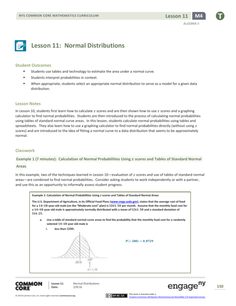
less than $𝟐𝟖𝟎.
𝑷(< 𝟐𝟖𝟎) = 𝟎. 𝟖𝟕𝟐𝟗
Lesson 11:
Date:
Normal Distributions
2/9/16
© 2014 Common Core, Inc. Some rights reserved. commoncore.org
150
This work is licensed under a
Creative Commons Attribution-NonCommercial-ShareAlike 3.0 Unported License.
Lesson 11
NYS COMMON CORE MATHEMATICS CURRICULUM
M4
ALGEBRA II
ii.
more than $𝟐𝟕𝟎
𝑷(> 𝟐𝟕𝟎) = 𝟏 − 𝟎. 𝟔𝟗𝟖𝟓
= 𝟎. 𝟑𝟎𝟏𝟓
iii.
more than $𝟐𝟓𝟎
𝑷(> 𝟐𝟓𝟎) = 𝟏 − 𝟎. 𝟐𝟑𝟖𝟗
= 𝟎. 𝟕𝟔𝟏𝟏
iv.
between $𝟐𝟒𝟎 and $𝟐𝟕𝟓
𝑷(between 𝟐𝟒𝟎 and 𝟐𝟕𝟓) = 𝟎. 𝟕𝟗𝟔𝟕 − 𝟎. 𝟎𝟗𝟑𝟒
= 𝟎. 𝟕𝟎𝟑𝟑
b.
Explain the meaning of the probability that you found in part (a–iv).
If a very large number of 𝟏𝟒−𝟏𝟖 year old males were to be selected at random, then you would expect about
𝟕𝟎. 𝟑𝟑% of them to have monthly food costs between $𝟐𝟒𝟎 and $𝟐𝟕𝟓.
Lesson 11:
Date:
Normal Distributions
2/9/16
© 2014 Common Core, Inc. Some rights reserved. commoncore.org
151
This work is licensed under a
Creative Commons Attribution-NonCommercial-ShareAlike 3.0 Unported License.
NYS COMMON CORE MATHEMATICS CURRICULUM
Lesson 11
M4
ALGEBRA II
Exercise 1 (5 minutes)
MP.4
This exercise provides practice with the approach demonstrated in Example 1. Continue to encourage students to
include a normal distribution curve with work shown for each part of the exercise.
Exercise 1
The USDA document described in Example 1 also states that the average cost of food for a 𝟏𝟒–𝟏𝟖 year old female (again,
on the “Moderate-cost” plan) is $𝟐𝟏𝟓. 𝟐𝟎 per month. Assume that the monthly food cost for a 𝟏𝟒–𝟏𝟖 year old female is
approximately normally distributed with mean $𝟐𝟏𝟓. 𝟐𝟎 and standard deviation $𝟏𝟒. 𝟖𝟓.
a.
Use a table of standard normal curve areas to find the probability that the monthly food cost for a randomly
selected 𝟏𝟒−𝟏𝟖 year old female is
i.
less than $𝟐𝟐𝟓.
𝑷(less than 𝟐𝟐𝟓) = 𝟎. 𝟕𝟒𝟓𝟒
ii.
less than $𝟐𝟎𝟎.
𝑷(less than 𝟐𝟎𝟎) = 𝟎. 𝟏𝟓𝟑𝟗
iii.
more than $𝟐𝟓𝟎.
𝑷(more than 𝟐𝟓𝟎) = 𝟎. 𝟎𝟎𝟗𝟔
Lesson 11:
Date:
Normal Distributions
2/9/16
© 2014 Common Core, Inc. Some rights reserved. commoncore.org
152
This work is licensed under a
Creative Commons Attribution-NonCommercial-ShareAlike 3.0 Unported License.
Lesson 11
NYS COMMON CORE MATHEMATICS CURRICULUM
M4
ALGEBRA II
iv.
between $𝟏𝟗𝟎 and $𝟐𝟐𝟎.
𝑷(between 𝟏𝟗𝟎 and 𝟐𝟐𝟎) = 𝟎. 𝟔𝟐𝟓𝟓 − 𝟎. 𝟎𝟒𝟒𝟔
= 𝟎. 𝟓𝟖𝟎𝟗
b.
Explain the meaning of the probability that you found in part (a–iv).
If a very large number of 𝟏𝟒–𝟏𝟖 year old females were to be selected at random, then you would expect about
𝟓𝟖. 𝟎𝟗% of them to have monthly food costs between $𝟏𝟗𝟎 and $𝟐𝟐𝟎.
Example 2 (5 minutes): Use of a Graphing Calculator to Find Normal Probabilities Directly
In this example, students learn how to calculate normal probabilities using a graphing calculator without using 𝑧 scores.
Use this example to show the class how to do this using a graphing calculator*.
*Calculator note: The general form of this is Normalcdf([left bound],[right bound],[mean],[standard deviation]). The
Normalcdf function is accessed using 2nd, DISTR.
Example 2: Use of a Graphing Calculator to Find Normal Probabilities Directly
Return to the information given in Example 1. Using a graphing calculator, and without using 𝒛 scores, find the
probability (rounded to the nearest thousandth) that the monthly food cost for a randomly selected 𝟏𝟒−𝟏𝟖 year old male
is
a.
between $𝟐𝟔𝟎 and $𝟐𝟔𝟓.
𝑷(between $𝟐𝟔𝟎 and $𝟐𝟔𝟓) = 𝟎. 𝟏𝟐𝟐.
If students are using TI-83 or
Normalcdf(𝟐𝟔𝟎, 𝟐𝟔𝟓, 𝟐𝟔𝟏. 𝟓, 𝟏𝟔. 𝟐𝟓).
b.
TI-84
calculators,
this
result
is
found
by
entering
at least $𝟐𝟓𝟐.
𝑷(≥ 𝟐𝟓𝟐) = 𝟎. 𝟕𝟐𝟏.
This result is found by entering Normalcdf(𝟐𝟓𝟐, 𝟗𝟗𝟗, 𝟐𝟔𝟏. 𝟓, 𝟏𝟔. 𝟐𝟓) or the equivalent for other brands of
calculator. Any large positive number or 1EE99 can be used in place of 𝟗𝟗𝟗, as long as the number is at least
four standard deviations above the mean.
c.
at most $𝟐𝟒𝟖.
𝑷(≤ 𝟐𝟒𝟖) = 𝟎. 𝟐𝟎𝟑
This result is found by entering Normalcdf(−𝟗𝟗𝟗, 𝟐𝟒𝟖, 𝟐𝟔𝟏. 𝟓, 𝟏𝟔. 𝟐𝟓) or the equivalent for other brands of
calculator. Any large negative number or –1EE99 can be used in place of −𝟗𝟗𝟗, as long as the number is at
least four standard deviations below the mean.
Lesson 11:
Date:
Normal Distributions
2/9/16
© 2014 Common Core, Inc. Some rights reserved. commoncore.org
153
This work is licensed under a
Creative Commons Attribution-NonCommercial-ShareAlike 3.0 Unported License.
Lesson 11
NYS COMMON CORE MATHEMATICS CURRICULUM
M4
ALGEBRA II
Exercise 2 (5 minutes)
MP.5 Here students have an opportunity to practice using a graphing calculator to find normal probabilities directly and reflect
on the use of technology compared to the use of tables of normal curve areas.
Exercise 2
Return to the information given in Exercise 1.
a.
In Exercise 1, you calculated the probability that the monthly food cost for a randomly selected 𝟏𝟒−𝟏𝟖 year
old female is between $𝟏𝟗𝟎 and $𝟐𝟐𝟎. Would the probability that that the monthly food cost for a randomly
selected 𝟏𝟒−𝟏𝟖 year old female is between $𝟏𝟗𝟓 and $𝟐𝟑𝟎 be greater than or smaller than the probability for
between $𝟏𝟗𝟎 and $𝟐𝟐𝟎? Explain your thinking.
The probability would be greater between $𝟏𝟗𝟓 and $𝟐𝟑𝟎. If you look at a sketch of a normal curve with
mean $𝟐𝟏𝟓. 𝟐𝟎 and standard deviation $𝟏𝟒. 𝟖𝟓, there is more area under the curve for the wider interval of
$𝟏𝟗𝟓 to $𝟐𝟑𝟎.
b.
Do you think that the probability that the monthly food cost for a randomly selected 𝟏𝟒−𝟏𝟖 year old female is
between $𝟏𝟗𝟓 and $𝟐𝟑𝟎 is closer to 𝟎. 𝟓𝟎, 𝟎. 𝟕𝟓, or 𝟎. 𝟗𝟎? Explain your thinking.
Closer to 𝟎. 𝟕𝟓. Based on my answer to part (a), I expect the probability to be greater than the probability for
between $𝟏𝟗𝟎 and $𝟐𝟐𝟎, which was 𝟎. 𝟓𝟖𝟎𝟗, but I do not think it would be as great as 𝟎. 𝟗𝟎.
c.
Using a graphing calculator, and without using 𝐳 scores, find the probability (rounded to the nearest
thousandth) that the monthly food cost for a randomly selected 𝟏𝟒−𝟏𝟖 year old female is between $𝟏𝟗𝟓
and $𝟐𝟑𝟎. Is this probability consistent with your answer to part (b)?
𝑷(between 𝟏𝟗𝟓 and 𝟐𝟑𝟎) = 𝟎. 𝟕𝟓𝟒
This probability is close to 𝟎. 𝟕𝟓, which was my answer in part (b).
d.
How does the probability you calculated in part (c) compare to the probability that would have been obtained
using the table of normal curve areas?
The z score for $𝟏𝟗𝟓 is 𝐳 =
𝟏𝟗𝟓−𝟐𝟏𝟓.𝟐𝟎
𝟐𝟑𝟎−𝟐𝟏𝟓.𝟐𝟎
= −𝟏. 𝟑𝟔, and the 𝐳 score for $𝟐𝟑𝟎 is 𝐳 =
= 𝟏. 𝟎𝟎. Using
𝟏𝟒.𝟖𝟓
𝟏𝟒.𝟖𝟓
the table of normal curve areas, 𝐏(between 𝟏𝟗𝟓 and 𝟐𝟑𝟎) = 𝟎. 𝟖𝟒𝟏𝟑 − 𝟎. 𝟎𝟖𝟓𝟑 = 𝟎. 𝟕𝟓𝟔. This is very close
to the answer I got using the graphing calculator.
e.
What is one advantage to using a graphing calculator to calculate this probability?
It is a lot faster to use the graphing calculator because I didn’t have to calculate 𝒛 scores in order to get the
probability.
f.
In Exercise 1, you calculated the probability that the monthly food cost for a randomly selected 𝟏𝟒–𝟏𝟖 year
old female is at most $𝟐𝟎𝟎. Would the probability that the monthly food cost for a randomly selected 𝟏𝟒–𝟏𝟖
year old female is at most $𝟐𝟏𝟎 be greater than or less than the probability for at most $𝟐𝟎𝟎? Explain your
thinking.
The probability would be greater for at most $𝟐𝟏𝟎. There is more area under the normal curve to the left of
$𝟐𝟏𝟎 than to the left of $𝟐𝟎𝟎.
g.
Do you think that the probability that the monthly food cost for a randomly selected 𝟏𝟒−𝟏𝟖 year old female is
at most $𝟐𝟏𝟎 is closer to 𝟎. 𝟏𝟎, 𝟎. 𝟑𝟎, or 𝟎. 𝟓𝟎? Explain your thinking.
Closer to 𝟎. 𝟑𝟎. Based on my answer to part (f), I expect the probability to be greater than the probability for
at most $𝟐𝟎𝟎, which was 𝟎. 𝟏𝟓𝟑𝟗, but I don’t think it would be as great as 𝟎. 𝟓𝟎 because $𝟐𝟏𝟎 is less than the
mean of $𝟐𝟏𝟓. 𝟐𝟎, and the area to the left of $𝟐𝟏𝟓. 𝟐𝟎 is 𝟎. 𝟓𝟎.
Lesson 11:
Date:
Normal Distributions
2/9/16
© 2014 Common Core, Inc. Some rights reserved. commoncore.org
154
This work is licensed under a
Creative Commons Attribution-NonCommercial-ShareAlike 3.0 Unported License.
Lesson 11
NYS COMMON CORE MATHEMATICS CURRICULUM
M4
ALGEBRA II
h.
Using a graphing calculator, and without using 𝒛 scores, find the probability (rounded to the nearest
thousandth) that the monthly food cost for a randomly selected 𝟏𝟒−𝟏𝟖 year old female is at most $𝟐𝟏𝟎.
𝑷(≤ 𝟐𝟏𝟎) = 𝟎. 𝟑𝟔𝟑
i.
Using a graphing calculator, and without using z scores, find the probability (rounded to the nearest
thousandth) that the monthly food cost for a randomly selected 𝟏𝟒−𝟏𝟖 year old female is at least $𝟐𝟑𝟓.
𝑷(≥ 𝟐𝟑𝟓) = 𝟎. 𝟎𝟗𝟏
Example 3 (5 minutes): Using a Spreadsheet to Find Normal Probabilities
In this example, students learn how to calculate normal probabilities using a spreadsheet. This example and the exercise
that follows revisits Example 1 and Exercise 1 but has students use a spreadsheet rather than a table of normal curve
areas. Use this example to show the class how to do this using a spreadsheet*.
*Spreadsheet note: Many spreadsheet programs, such as Excel, have a built in function to calculate normal
probabilities. In Excel, this can be done by finding the area to the left of any particular cutoff value by typing the
following into a cell of the spreadsheet and then hitting the return key:
= NORMDIST(cutoff,mean,stddev,true).
You need to include the true at the end in order to get the area to the left of the cutoff. For example,
= NORMDIST(50,40,10,true) will give 0.84124, which is the area to the left of 50 under the normal curve with
mean 40 and standard deviation 10.
Example 3: Using a Spreadsheet to Find Normal Probabilities
Return to the information given in Example 1. The U.S. Department of Agriculture, in its Official Food Plans
(www.cnpp.usda.gov), states that the average cost of food for a 𝟏𝟒–𝟏𝟖-year-old male (on the “moderate-cost” plan) is
$𝟐𝟔𝟏. 𝟓𝟎 per month. Assume that the monthly food cost for a 𝟏𝟒–𝟏𝟖-year-old male is approximately normally
distributed with a mean of $𝟐𝟔𝟏. 𝟓𝟎 and a standard deviation of $𝟏𝟔. 𝟐𝟓. Round your answers to four decimal places.
Use a spreadsheet to find the probability that the monthly food cost for a randomly selected 𝟏𝟒−𝟏𝟖 year old male is
a.
less than $𝟐𝟖𝟎.
If students are using Excel, this would be found by using
=NORMDIST(𝟐𝟖𝟎, 𝟐𝟔𝟏. 𝟓𝟎, 𝟏𝟔. 𝟐𝟓, true). The difference
between this answer and the answer using the table of
normal curve areas is due to rounding in calculating the 𝒛
score needed in order to use the table.
𝑷(< 𝟐𝟖𝟎) = 𝟎. 𝟖𝟕𝟐𝟓
b.
more than $𝟐𝟕𝟎.
𝑷(> 𝟐𝟕𝟎) = 𝟏 − 𝟎. 𝟔𝟗𝟗𝟓
= 𝟎. 𝟑𝟎𝟎𝟓
Lesson 11:
Date:
Normal Distributions
2/9/16
© 2014 Common Core, Inc. Some rights reserved. commoncore.org
155
This work is licensed under a
Creative Commons Attribution-NonCommercial-ShareAlike 3.0 Unported License.
Lesson 11
NYS COMMON CORE MATHEMATICS CURRICULUM
M4
ALGEBRA II
c.
more than $𝟐𝟓𝟎.
𝑷(> 𝟐𝟓𝟎) = 𝟏 − 𝟎. 𝟐𝟑𝟗𝟔
= 𝟎. 𝟕𝟔𝟎𝟒
d.
between $𝟐𝟒𝟎 and $𝟐𝟕𝟓.
𝑷(between 𝟐𝟒𝟎 and 𝟐𝟕𝟓) = 𝟎. 𝟕𝟗𝟔𝟗 − 𝟎. 𝟎𝟗𝟐𝟗
= 𝟎. 𝟕𝟎𝟒𝟎
Exercise 3 (5 minutes)
Exercise 3
The USDA document described in Example 1 also states that the average cost of food for a 𝟏𝟒–𝟏𝟖 year old female (again,
on the “moderate-cost” plan) is $𝟐𝟏𝟓. 𝟐𝟎 per month. Assume that the monthly food cost for a 𝟏𝟒–𝟏𝟖 year old female is
approximately normally distributed with a mean of $𝟐𝟏𝟓. 𝟐𝟎 and a standard deviation of $𝟏𝟒. 𝟖𝟓. Round your answers
to 𝟒 decimal places.
Use a spreadsheet to find the probability that the monthly food cost for a randomly selected 𝟏𝟒−𝟏𝟖 year old female is
a.
less than $𝟐𝟐𝟓.
𝑷(less than 𝟐𝟐𝟓) = 𝟎. 𝟕𝟒𝟓𝟒
b.
less than $𝟐𝟎𝟎.
𝑷(less than 𝟐𝟎𝟎) = 𝟎. 𝟏𝟓𝟑𝟎
Lesson 11:
Date:
Normal Distributions
2/9/16
© 2014 Common Core, Inc. Some rights reserved. commoncore.org
156
This work is licensed under a
Creative Commons Attribution-NonCommercial-ShareAlike 3.0 Unported License.
NYS COMMON CORE MATHEMATICS CURRICULUM
Lesson 11
M4
ALGEBRA II
c.
more than $𝟐𝟓𝟎.
𝑷(𝒎𝒐𝒓𝒆 𝒕𝒉𝒂𝒏 𝟐𝟓𝟎) = 𝟏 − 𝟎. 𝟗𝟗𝟎𝟒
= 𝟎. 𝟎𝟎𝟗𝟔
d.
between $𝟏𝟗𝟎 and $𝟐𝟐𝟎.
𝑷(between 𝟏𝟗𝟎 and 𝟐𝟐𝟎) = 𝟎. 𝟔𝟐𝟔𝟕 − 𝟎. 𝟎𝟒𝟒𝟗
= 𝟎. 𝟓𝟖𝟏𝟖
Exercise 4 (6 minutes)
Here students are led through the process of choosing a normal distribution to model a given data set. Students might
need some assistance prior to tackling this exercise. Teachers may wish to provide a quick review of how to draw a
histogram. Students may need to be reminded how to calculate the mean and the standard deviation for data given in
the form of a frequency distribution. In fact, this example provides the additional complication that the data are given in
the form of a grouped frequency distribution, so the midpoints of the intervals have to be used as the data values.
If time is short you can simply provide students with reminders of these techniques mentioned above, and the exercise
can then be finished as part of the homework assignment.
Lesson 11:
Date:
Normal Distributions
2/9/16
© 2014 Common Core, Inc. Some rights reserved. commoncore.org
157
This work is licensed under a
Creative Commons Attribution-NonCommercial-ShareAlike 3.0 Unported License.
Lesson 11
NYS COMMON CORE MATHEMATICS CURRICULUM
M4
ALGEBRA II
Exercise 4
The reaction times of 𝟒𝟗𝟎 people were measured. The results are shown in the frequency distribution below.
Reaction Time
(seconds)
Frequency
𝟎. 𝟏 to < 𝟎. 𝟏𝟓
𝟎. 𝟏𝟓 to < 𝟎. 𝟐
𝟎. 𝟐 to < 𝟎. 𝟐𝟓
𝟎. 𝟐𝟓 to < 𝟎. 𝟑
𝟎. 𝟑 to < 𝟎. 𝟑𝟓
𝟎. 𝟑𝟓 to < 𝟎. 𝟒
𝟗
𝟖𝟐
𝟐𝟐𝟎
𝟏𝟑𝟖
𝟑𝟕
𝟒
a.
Construct a histogram that displays these results.
b.
Looking at the histogram, do you think a normal distribution would be an appropriate model for this distribution?
Yes, the histogram is approximately symmetric and mound shaped.
c.
The mean of the reaction times for these 𝟒𝟗𝟎 people is 𝟎. 𝟐𝟑𝟕𝟕, and the standard deviation of the reaction times
is 𝟎. 𝟎𝟒𝟓𝟕. For a normal distribution with this mean and standard deviation, what is the probability that a
randomly selected reaction time is at least 𝟎. 𝟐𝟓?
Using Normalcdf(𝟎. 𝟐𝟓, 𝟗𝟗𝟗, 𝟎. 𝟐𝟑𝟕𝟕, 𝟎. 𝟎𝟒𝟓𝟕), you get 𝑷(≥ 𝟎. 𝟐𝟓) = 𝟎. 𝟑𝟗𝟒.
d.
The actual proportion of these 𝟒𝟗𝟎 people who had a reaction time that was at least 𝟎. 𝟐𝟓 is 𝟎. 𝟑𝟔𝟓 (this can be
calculated from the frequency distribution). How does this proportion compare to the probability that you
calculated in part (c)? Does this confirm that the normal distribution is an appropriate model for the reaction time
distribution?
𝟎. 𝟑𝟔𝟓 is reasonably close to the probability based on the normal distribution, which was 𝟎. 𝟑𝟗𝟒. I think that the
normal model was appropriate.
Closing (2 minutes)
Refer to Exercise 3.

How would you interpret the probability that you found using a calculator in part (c)?

Approximately 39.4% of the people had a reaction time of 0.25 seconds or higher.
Ask students to summarize the main ideas of the lesson in writing or with a neighbor. Use this as an opportunity to
informally assess comprehension of the lesson. The Lesson Summary below offers some important ideas that should be
included.
Lesson 11:
Date:
Normal Distributions
2/9/16
© 2014 Common Core, Inc. Some rights reserved. commoncore.org
158
This work is licensed under a
Creative Commons Attribution-NonCommercial-ShareAlike 3.0 Unported License.
NYS COMMON CORE MATHEMATICS CURRICULUM
Lesson 11
M4
ALGEBRA II
Lesson Summary
Probabilities associated with normal distributions can be found using 𝒛 scores and tables of standard normal curve
areas.
Probabilities associated with normal distributions can be found directly (without using 𝒛 scores) using a graphing
calculator.
When a data distribution has a shape that is approximately normal, a normal distribution can be used as a model
for the data distribution. The normal distribution with the same mean and the standard deviation as the data
distribution is used.
Exit Ticket (5 minutes)
Lesson 11:
Date:
Normal Distributions
2/9/16
© 2014 Common Core, Inc. Some rights reserved. commoncore.org
159
This work is licensed under a
Creative Commons Attribution-NonCommercial-ShareAlike 3.0 Unported License.
Lesson 11
NYS COMMON CORE MATHEMATICS CURRICULUM
M4
ALGEBRA II
Name
Date
Lesson 11: Normal Distributions
Exit Ticket
1.
2.
SAT scores were originally scaled so that the scores for each section were approximately normally distributed with a
mean of 500 and a standard deviation of 100. Assuming that this scaling still applies, use a table of standard normal
curve areas to find the probability that a randomly selected SAT student scores
a.
more than 700.
b.
between 440 and 560.
In 2012 the mean SAT math score was 514, and the standard deviation was 117. For the purposes of this question,
assume that the scores were normally distributed. Using a graphing calculator, and without using 𝑧 scores, find the
probability (rounded to the nearest thousandth), and explain how the answer was determined that a randomly
selected SAT math student in 2012 scored
a.
between 400 and 480.
b.
less than 350.
Lesson 11:
Date:
Normal Distributions
2/9/16
© 2014 Common Core, Inc. Some rights reserved. commoncore.org
160
This work is licensed under a
Creative Commons Attribution-NonCommercial-ShareAlike 3.0 Unported License.
Lesson 11
NYS COMMON CORE MATHEMATICS CURRICULUM
M4
ALGEBRA II
Exit Ticket Sample Solutions
SAT scores were originally scaled so that the scores for each section were approximately normally distributed with a
mean of 𝟓𝟎𝟎 and a standard deviation of 𝟏𝟎𝟎. Assuming that this scaling still applies, use a table of standard
normal curve areas to find the probability that a randomly selected SAT student scores
a.
more than 𝟕𝟎𝟎.
𝑷(> 𝟕𝟎𝟎) = 𝟏 − 𝟎. 𝟗𝟕𝟕𝟐
= 𝟎. 𝟎𝟐𝟐𝟖
b.
between 𝟒𝟒𝟎 and 𝟓𝟔𝟎.
𝑷(between 𝟒𝟒𝟎 and 𝟓𝟔𝟎) = 𝟎. 𝟕𝟐𝟓𝟕 − 𝟎. 𝟐𝟕𝟒𝟑
= 𝟎. 𝟒𝟓𝟏𝟒
In 2012 the mean SAT math score was 𝟓𝟏𝟒 and the standard deviation was 𝟏𝟏𝟕. For the purposes of this question,
assume that the scores were normally distributed. Using a graphing calculator, and without using 𝒛 scores, find the
probability (rounded to the nearest thousandth), and explain how the answer was determined that a randomly
selected SAT math student in 2012 scored
a.
between 𝟒𝟎𝟎 and 𝟒𝟖𝟎.
𝑷(between 𝟒𝟎𝟎 and 𝟒𝟖𝟎) = 𝟎. 𝟐𝟐𝟏
I used a TI-84 graphing calculator: Normalcdf(𝟒𝟎𝟎, 𝟒𝟖𝟎, 𝟓𝟏𝟒, 𝟏𝟏𝟕).
b.
less than 𝟑𝟓𝟎.
𝑷(< 𝟑𝟓𝟎) = 𝟎. 𝟎𝟖𝟏
I used a TI-84 graphing calculator: Normalcdf(𝟎, 𝟑𝟓𝟎, 𝟓𝟏𝟒, 𝟏𝟏𝟕).
Lesson 11:
Date:
Normal Distributions
2/9/16
© 2014 Common Core, Inc. Some rights reserved. commoncore.org
161
This work is licensed under a
Creative Commons Attribution-NonCommercial-ShareAlike 3.0 Unported License.
Lesson 11
NYS COMMON CORE MATHEMATICS CURRICULUM
M4
ALGEBRA II
Problem Set Sample Solutions
Use a table of standard normal curve areas to find
a.
the area to the left of 𝒛 = 𝟏. 𝟖𝟖.
𝟎. 𝟗𝟔𝟗𝟗
b.
the area to the right of 𝒛 = 𝟏. 𝟒𝟐.
𝟏 − 𝟎. 𝟗𝟐𝟐𝟐 = 𝟎. 𝟎𝟕𝟕𝟖
c.
the area to the left of 𝒛 = −𝟎. 𝟑𝟗.
𝟎. 𝟑𝟒𝟖𝟑
d.
the area to the right of 𝒛 = −𝟎. 𝟒𝟔.
𝟏 − 𝟎. 𝟑𝟐𝟐𝟖 = 𝟎. 𝟔𝟕𝟕𝟐
e.
the area between 𝒛 = −𝟏. 𝟐𝟐 and 𝒛 = −𝟎. 𝟓.
𝟎. 𝟑𝟎𝟖𝟓 − 𝟎. 𝟏𝟏𝟏𝟐 = 𝟎. 𝟏𝟗𝟕𝟑
Suppose that the durations of high school baseball games are approximately normally distributed with mean 𝟏𝟎𝟓
minutes and standard deviation 𝟏𝟏 minutes. Use a table of standard normal curve areas to find the probability that
a randomly selected high school baseball game lasts
a.
less than 𝟏𝟏𝟓 minutes.
𝑷(< 𝟏𝟏𝟓) = 𝟎. 𝟖𝟏𝟖𝟔
b.
more than 𝟏𝟎𝟎 minutes.
𝑷(> 𝟏𝟎𝟎) = 𝟏 − 𝟎. 𝟑𝟐𝟔𝟒
= 𝟎. 𝟔𝟕𝟑𝟔
Lesson 11:
Date:
Normal Distributions
2/9/16
© 2014 Common Core, Inc. Some rights reserved. commoncore.org
162
This work is licensed under a
Creative Commons Attribution-NonCommercial-ShareAlike 3.0 Unported License.
NYS COMMON CORE MATHEMATICS CURRICULUM
Lesson 11
M4
ALGEBRA II
c.
between 𝟗𝟎 and 𝟏𝟏𝟎 minutes.
𝑷(between 𝟗𝟎 and 𝟏𝟏𝟎) = 𝟎. 𝟔𝟕𝟑𝟔 − 𝟎. 𝟎𝟖𝟔𝟗
= 𝟎. 𝟓𝟖𝟔𝟕
Using a graphing calculator, and without using 𝒛 values, check your answers to Problem 2. (Round your answers to
the nearest thousandth.)
a.
𝑷(< 𝟏𝟏𝟓) = 𝟎. 𝟖𝟏𝟖
b.
𝑷(> 𝟏𝟎𝟎) = 𝟎. 𝟔𝟕𝟓
c.
𝑷(between 𝟗𝟎 and 𝟏𝟏𝟎) = 𝟎. 𝟓𝟖𝟗
In Problem 2, you were told that the durations of high school baseball games are approximately normally
distributed with mean 𝟏𝟎𝟓 minutes and standard deviation 𝟏𝟏 minutes. Suppose also that the durations of high
school softball games are approximately normally distributed with a mean of 𝟗𝟓 minutes and the same standard
deviation, 𝟏𝟏 minutes. Is it more likely that a high school baseball game will last between 𝟏𝟎𝟎 and 𝟏𝟏𝟎 minutes or
that a high school softball game will last between 𝟏𝟎𝟎 and 𝟏𝟏𝟎 minutes? Answer this question without doing any
calculations!
The heights of the two normal distribution graphs are the same; the only difference between the graphs is that the
softball graph has a smaller mean. So when the region under the graph between 𝟏𝟎𝟎 and 𝟏𝟏𝟎 is shaded, you get a
larger area for the baseball graph than for the softball graph. Therefore, it is more likely that the baseball game
will last between 𝟏𝟎𝟎 and 𝟏𝟏𝟎 minutes.
Lesson 11:
Date:
Normal Distributions
2/9/16
© 2014 Common Core, Inc. Some rights reserved. commoncore.org
163
This work is licensed under a
Creative Commons Attribution-NonCommercial-ShareAlike 3.0 Unported License.
Lesson 11
NYS COMMON CORE MATHEMATICS CURRICULUM
M4
ALGEBRA II
A farmer has 𝟔𝟐𝟓 female adult sheep. The sheep have recently been weighed, and the results are shown in the
table below.
Weight
(pounds)
Frequency
𝟏𝟒𝟎 to <
𝟏𝟓𝟎
𝟖
𝟏𝟓𝟎 to <
𝟏𝟔𝟎
𝟑𝟔
𝟏𝟔𝟎 to <
𝟏𝟕𝟎
𝟏𝟕𝟑
𝟏𝟕𝟎 to <
𝟏𝟖𝟎
𝟐𝟐𝟏
𝟏𝟖𝟎 to <
𝟏𝟗𝟎
𝟏𝟒𝟗
𝟏𝟗𝟎 to <
𝟐𝟎𝟎
𝟑𝟑
𝟐𝟎𝟎 to <
𝟐𝟏𝟎
𝟓
a.
Construct a histogram that displays these results.
b.
Looking at the histogram, do you think a normal distribution would be an appropriate model for this
distribution?
Yes. The histogram is approximately symmetric and mound shaped.
c.
The weights of the 𝟔𝟐𝟓 sheep have mean 𝟏𝟕𝟒. 𝟐𝟏 pounds and standard deviation 𝟏𝟎. 𝟏𝟏 pounds. For a
normal distribution with this mean and standard deviation, what is the probability that a randomly selected
sheep has a weight of at least 𝟏𝟗𝟎 pounds? (Round your answer to the nearest thousandth.)
Using Normalcdf(𝟏𝟗𝟎, 𝟗𝟗𝟗, 𝟏𝟕𝟒. 𝟐𝟏, 𝟏𝟎. 𝟏𝟏), you get 𝑷(≥ 𝟏𝟗𝟎) = 𝟎. 𝟎𝟓𝟗.
Lesson 11:
Date:
Normal Distributions
2/9/16
© 2014 Common Core, Inc. Some rights reserved. commoncore.org
164
This work is licensed under a
Creative Commons Attribution-NonCommercial-ShareAlike 3.0 Unported License.
Lesson 11
NYS COMMON CORE MATHEMATICS CURRICULUM
M4
ALGEBRA II
Standard Normal Curve Areas
z
–3.8
–3.7
–3.6
–3.5
–3.4
–3.3
–3.2
–3.1
–3.0
–2.9
–2.8
–2.7
–2.6
–2.5
–2.4
–2.3
–2.2
–2.1
–2.0
–1.9
–1.8
–1.7
–1.6
–1.5
–1.4
–1.3
–1.2
–1.1
–1.0
–0.9
–0.8
–0.7
–0.6
–0.5
–0.4
–0.3
–0.2
–0.1
–0.0
0.00
0.0001
0.0001
0.0002
0.0002
0.0003
0.0005
0.0007
0.0010
0.0013
0.0019
0.0026
0.0035
0.0047
0.0062
0.0082
0.0107
0.0139
0.0179
0.0228
0.0287
0.0359
0.0446
0.0548
0.0668
0.0808
0.0968
0.1151
0.1357
0.1587
0.1841
0.2119
0.2420
0.2743
0.3085
0.3446
0.3821
0.4207
0.4602
0.5000
0.01
0.0001
0.0001
0.0002
0.0002
0.0003
0.0005
0.0007
0.0009
0.0013
0.0018
0.0025
0.0034
0.0045
0.0060
0.0080
0.0104
0.0136
0.0174
0.0222
0.0281
0.0351
0.0436
0.0537
0.0655
0.0793
0.0951
0.1131
0.1335
0.1562
0.1814
0.2090
0.2389
0.2709
0.3050
0.3409
0.3783
0.4168
0.4562
0.4960
Lesson 11:
Date:
0.02
0.0001
0.0001
0.0001
0.0002
0.0003
0.0005
0.0006
0.0009
0.0013
0.0018
0.0024
0.0033
0.0044
0.0059
0.0078
0.0102
0.0132
0.0160
0.0217
0.0274
0.0344
0.0427
0.0526
0.0643
0.0778
0.0934
0.1112
0.1314
0.1539
0.1788
0.2061
0.2358
0.2676
0.3015
0.3372
0.3745
0.4129
0.4522
0.4920
0.03
0.0001
0.0001
0.0001
0.0002
0.0003
0.0004
0.0006
0.0009
0.0012
0.0017
0.0023
0.0032
0.0043
0.0057
0.0075
0.0099
0.0129
0.0166
0.0212
0.0268
0.0336
0.0418
0.0516
0.0630
0.0764
0.0918
0.1093
0.1292
0.1515
0.1762
0.2033
0.2327
0.2643
0.2981
0.3336
0.3707
0.4090
0.4483
0.4880
0.04
0.0001
0.0001
0.0001
0.0002
0.0003
0.0004
0.0006
0.0008
0.0012
0.0016
0.0023
0.0031
0.0041
0.0055
0.0073
0.0096
0.0125
0.0162
0.0207
0.0262
0.0329
0.0409
0.0505
0.0618
0.0749
0.0901
0.1075
0.1271
0.1492
0.1736
0.2005
0.2296
0.2611
0.2946
0.3300
0.3669
0.4052
0.4443
0.4840
0.05
0.0001
0.0001
0.0001
0.0002
0.0003
0.0004
0.0006
0.0008
0.0011
0.0016
0.0022
0.0030
0.0040
0.0054
0.0071
0.0094
0.0122
0.0158
0.0202
0.0256
0.0322
0.0401
0.0495
0.0606
0.0735
0.0885
0.1056
0.1251
0.1469
0.1711
0.1977
0.2266
0.2578
0.2912
0.3264
0.3632
0.4013
0.4404
0.4801
0.06
0.0001
0.0001
0.0001
0.0002
0.0003
0.0004
0.0006
0.0008
0.0011
0.0015
0.0021
0.0029
0.0039
0.0052
0.0069
0.0091
0.0119
0.0154
0.0197
0.0250
0.0314
0.0392
0.0485
0.0594
0.0721
0.0869
0.1038
0.1230
0.1446
0.1685
0.1949
0.2236
0.2546
0.2877
0.3228
0.3594
0.3974
0.4364
0.4761
0.07
0.0001
0.0001
0.0001
0.0002
0.0003
0.0004
0.0005
0.0008
0.0011
0.0015
0.0021
0.0028
0.0038
0.0051
0.0068
0.0089
0.0116
0.0150
0.0192
0.0244
0.0307
0.0384
0.0475
0.0582
0.0708
0.0853
0.1020
0.1210
0.1423
0.1660
0.1922
0.2206
0.2514
0.2843
0.3192
0.3557
0.3936
0.4325
0.4721
0.08
0.0001
0.0001
0.0001
0.0002
0.0003
0.0004
0.0005
0.0007
0.0010
0.0014
0.0020
0.0027
0.0037
0.0049
0.0066
0.0087
0.0113
0.0146
0.0188
0.0239
0.0301
0.0375
0.0465
0.0571
0.0694
0.0838
0.1003
0.1190
0.1401
0.1635
0.1894
0.2177
0.2483
0.2810
0.3156
0.3520
0.3897
0.4286
0.4681
0.09
0.0001
0.0001
0.0001
0.0002
0.0002
0.0003
0.0005
0.0007
0.0010
0.0014
0.0019
0.0026
0.0036
0.0048
0.0064
0.0084
0.0110
0.0143
0.0183
0.0233
0.0294
0.0367
0.0455
0.0599
0.0681
0.0823
0.0985
0.1170
0.1379
0.1611
0.1867
0.2148
0.2451
0.2776
0.3121
0.3483
0.3859
0.4247
0.4641
Normal Distributions
2/9/16
© 2014 Common Core, Inc. Some rights reserved. commoncore.org
165
This work is licensed under a
Creative Commons Attribution-NonCommercial-ShareAlike 3.0 Unported License.
Lesson 11
NYS COMMON CORE MATHEMATICS CURRICULUM
M4
ALGEBRA II
z
0.0
0.1
0.2
0.3
0.4
0.5
0.6
0.7
0.8
0.9
1.0
1.1
1.2
1.3
1.4
1.5
1.6
1.7
1.8
1.9
2.0
2.1
2.2
2.3
2.4
2.5
2.6
2.7
2.8
2.9
3.0
3.1
3.2
3.3
3.4
3.5
3.6
3.7
3.8
0.00
0.5000
0.5398
0.5793
0.6179
0.6554
0.6915
0.7257
0.7580
0.7881
0.8159
0.8413
0.8643
0.8849
0.9032
0.9192
0.9332
0.9452
0.9554
0.9641
0.9713
0.9772
0.9821
0.9861
0.9893
0.9918
0.9938
0.9953
0.9965
0.9974
0.9981
0.9987
0.9990
0.9993
0.9995
0.9997
0.9998
0.9998
0.9999
0.9999
0.01
0.5040
0.5438
0.5832
0.6217
0.6591
0.6950
0.7291
0.7611
0.7910
0.8186
0.8438
0.8665
0.8869
0.9049
0.9207
0.9345
0.9463
0.9564
0.9649
0.9719
0.9778
0.9826
0.9864
0.9896
0.9920
0.9940
0.9955
0.9966
0.9975
0.9982
0.9987
0.9991
0.9993
0.9995
0.9997
0.9998
0.9998
0.9999
0.9999
Lesson 11:
Date:
0.02
0.5080
0.5478
0.5871
0.6255
0.6628
0.6985
0.7324
0.7642
0.7939
0.8212
0.8461
0.8686
0.8888
0.9066
0.9222
0.9357
0.9474
0.9573
0.9656
0.9726
0.9783
0.9830
0.9868
0.9898
0.9922
0.9941
0.9956
0.9967
0.9976
0.9982
0.9987
0.9991
0.9994
0.9995
0.9997
0.9998
0.9999
0.9999
0.9999
0.03
0.5120
0.5517
0.5910
0.6293
0.6664
0.7019
0.7357
0.7673
0.7967
0.8238
0.8485
0.8708
0.8907
0.9082
0.9236
0.9370
0.9484
0.9582
0.9664
0.9732
0.9788
0.9834
0.9871
0.9901
0.9925
0.9943
0.9957
0.9968
0.9977
0.9983
0.9988
0.9991
0.9994
0.9996
0.9997
0.9998
0.9999
0.9999
0.9999
0.04
0.5160
0.5557
0.5948
0.6331
0.6700
0.7054
0.7389
0.7704
0.7995
0.8264
0.8508
0.8729
0.8925
0.9099
0.9251
0.9382
0.9495
0.9591
0.9671
0.9738
0.9793
0.9838
0.9875
0.9904
0.9927
0.9945
0.9959
0.9969
0.9977
0.9984
0.9988
0.9992
0.9994
0.9996
0.9997
0.9998
0.9999
0.9999
0.9999
0.05
0.5199
0.5596
0.5987
0.6368
0.6736
0.7088
0.7422
0.7734
0.8023
0.8289
0.8531
0.8749
0.8944
0.9115
0.9265
0.9394
0.9505
0.9599
0.9678
0.9744
0.9798
0.9842
0.9878
0.9906
0.9929
0.9946
0.9960
0.9970
0.9978
0.9984
0.9989
0.9992
0.9994
0.9996
0.9997
0.9998
0.9999
0.9999
0.9999
0.06
0.5239
0.5636
0.6026
0.6406
0.6772
0.7123
0.7454
0.7764
0.8051
0.8315
0.8554
0.8770
0.8962
0.9131
0.9279
0.9406
0.9515
0.9608
0.9686
0.9750
0.9803
0.9846
0.9881
0.9909
0.9931
0.9948
0.9961
0.9971
0.9979
0.9985
0.9989
0.9992
0.9994
0.9996
0.9997
0.9998
0.9999
0.9999
0.9999
0.07
0.5279
0.5675
0.6064
0.6443
0.6808
0.7157
0.7486
0.7794
0.8078
0.8340
0.8577
0.8790
0.8980
0.9147
0.9292
0.9418
0.9525
0.9616
0.9693
0.9756
0.9808
0.9850
0.9884
0.9911
0.9932
0.9949
0.9962
0.9972
0.9979
0.9985
0.9989
0.9992
0.9995
0.9996
0.9997
0.9998
0.9999
0.9999
0.9999
0.08
0.5319
0.5714
0.6103
0.6480
0.6844
0.7190
0.7517
0.7823
0.8106
0.8365
0.8599
0.8810
0.8997
0.9162
0.9306
0.9429
0.9535
0.9625
0.9699
0.9761
0.9812
0.9854
0.9887
0.9913
0.9934
0.9951
0.9963
0.9973
0.9980
0.9986
0.9990
0.9993
0.9995
0.9996
0.9997
0.9998
0.9999
0.9999
0.9999
0.09
0.5359
0.5753
0.6141
0.6517
0.6879
0.7224
0.7549
0.7852
0.8133
0.8389
0.8621
0.8830
0.9015
0.9177
0.9319
0.9441
0.9545
0.9633
0.9706
0.9767
0.9817
0.9857
0.9890
0.9916
0.9936
0.9952
0.9964
0.9974
0.9981
0.9986
0.9990
0.9993
0.9995
0.9997
0.9998
0.9998
0.9999
0.9999
0.9999
Normal Distributions
2/9/16
© 2014 Common Core, Inc. Some rights reserved. commoncore.org
166
This work is licensed under a
Creative Commons Attribution-NonCommercial-ShareAlike 3.0 Unported License.