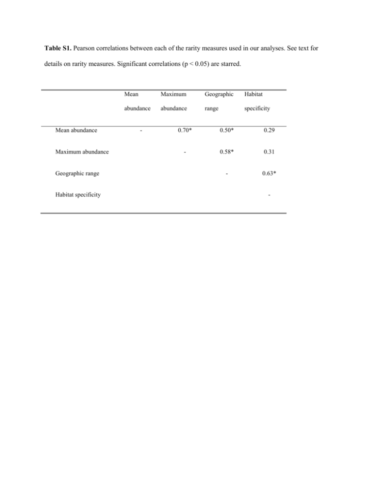
Table S1. Pearson correlations between each of the rarity measures used in our analyses. See text for
details on rarity measures. Significant correlations (p < 0.05) are starred.
Mean abundance
Maximum abundance
Geographic range
Habitat specificity
Mean
Maximum
Geographic
Habitat
abundance
abundance
range
specificity
-
0.70*
0.50*
0.29
-
0.58*
0.31
-
0.63*
-
Table S2. Sensitivity analysis examining all three-trait combinations from the four traits used in our
analyses. The slope of the regression as well as its p value from the bootstrapped analysis are reported
(significance at  = 0.05 marked with **, at  = 0.1 marked with *). Rare species significantly contribute
less to FTV than more common species when rarity is defined by mean abundance (p < 0.10). There is
some evidence that plant mass influenced our results since rare species contributed less to FTV when
rarity was defined by maximum abundance and geographic range (p < 0.10), however, there was still
higher significance when rarity was defined by mean abundance (p < .05).
Trait removed from
analysis
Rarity metric
Leaf mass
Mean abundance
-0.0024
0.025**
Maximum abundance
-0.0004
0.344
Geographic range
-0.0005
0.343
Habitat specificity
-0.0005
0.341
Mean abundance
-0.0007
0.061*
Maximum abundance
-0.0006
0.100
Geographic range
0.0002
0.341
Habitat specificity
-0.0002
0.346
Mean abundance
-0.0006
0.008**
Maximum abundance
-0.0004
0.080*
Geographic range
-0.0004
0.061*
Habitat specificity
-0.0001
0.342
Mean abundance
-0.0015
0.049**
Maximum abundance
-0.0010
0.140
Geographic range
-0.0005
0.331
Habitat specificity
-0.0014
0.102
Root to shoot ratio
Plant mass
Leaf nitrogen
content
Slope of regression
Bootstrap p value
Table S3. Species names for all 46 species that were considered in our analyses. Rarity rank of each of
the four measures of rarity for each of our species is listed, where 1 equals the most common, 46 equals
the most rare, and NA identifies species-rarity rank combinations where data were unavailable.
Habitat
Specificity
Rank
19
Geographic
Abundance
Rank
3
Mean
Abundance
Rank
13
Max
Abundance
Rank
30
Agrostis scabra
NA
10
14
13
Ambrosia artemisiifolia
15
9
8
12
Ambrosia psilostachya
15
23
23
29
Andropogon gerardii
29
25
4
7
Anemone cylindrica
35
37
31
16
Aristida basiramea
19
40
30
41
Artemisa campestris
15
22
36
34
Artemisia ludoviciana
15
20
27
24
Berteroa incana
15
28
9
14
Boechera grahamii
39
37
37
45
Bromus inermis
15
7
24
19
Carex sp.
25
NA
5
6
Crepis tectorum
NA
3
10
20
Digitaria cognata
25
37
39
37
Dichanthelium oligosanthes
31
21
16
32
Dichanthelium perlongum
39
28
32
25
Dichanthelium acuminatum var.
acuminatum
39
31
33
27
Elytrigia repens
15
11
3
8
Erigeron canadensis
NA
32
12
15
Erigeron strigosus
19
17
38
44
Fragaria virginiana
19
5
25
9
Hedeoma hispidum
33
29
22
43
Helianthus sp.
NA
NA
46
42
Hesperostipa spartea
41
42
28
19
Koeleria macrantha
41
28
43
38
Lathyrus venosus
35
34
26
33
Lespedeza capitata
29
33
20
28
Lithospermum caroliniense
39
38
42
35
Species Name
Achillea millefolium
Monarda fistulosa
22
20
35
31
Physalis virginiana
33
31
34
36
Poa pratensis
15
1
1
2
Polygonum convolvulus
15
5
19
10
Potentilla recta
15
16
44
23
Rosa arkansana
25
40
21
26
Rubus sp.
NA
NA
18
4
Rumex acetosella
15
6
7
21
Schizachyrium scoparium
29
16
2
1
Silene latifolia
22
20
17
39
Solidago gigantea
22
12
11
5
Sorghastrum nutans
29
25
15
18
Stachys palustris
31
41
40
40
Tragopogon dubius
15
43
45
46
Tradescantia occidentalis
15
14
29
17
Verbascum thapsus
15
9
41
22
Vicia villosa
15
14
6
3
Figure S1. Unscaled rank-abundance plots of the 248 plant species present in the Cedar Creek oldfield
survey, showing mean abundance for each species; error bars are ± 1 s.e. Species for which we have trait
data, and are thus included in our analyses, are highlighted in red. Species are ranked from the most
common to the most rare. Our analyses included 28 species that had mean abundances less than 10% of
the 10 most common species, and 18 species that had mean abundances less than 5% of the 10 most
common species suggesting that we covered a wide range of rarity ranks in our study.
-
Species in oldfield survey
Species with trait data
+/- 1 s.e. of mean percent cover
6
4
-
2
----------------------------------------------------------------------------------------------------------------------
0
Percent cover
8
10
-
0
50
100
150
Rank
200
250
Figure S2. Pearson correlation coefficients (r) between the four traits considered in our study: leaf
nitrogen, leaf mass per area (LMA), root to shoot ratio, and plant mass. Histograms of each trait are on
the diagonal, scatterplots of the two-way pairings of traits are in the upper-right, and correlation values
are in the bottom-left. Significant correlations are in bold.
Figure S3. Summary of principal component analysis of the four selected traits across the 46 species. The
first principal component (PC1) represents part of the leaf economics spectrum, with leaf mass per area
(LMA) and leaf nitrogen concentration (pctN.leaves) negatively correlated with each other; this axis
represented 47.7% of the variance (bottom right panel). Plant size (plantmass) was partially correlated
with LMA for these grassland plants. PC2 separates plants along a root investment gradient, with
graminoids at the high end; this axis represents and additional 26.9% of the variance. PC3 is driven
mostly by plant size and captures 18.1% of the variance, for a total of 90.5% of the variation in these
three orthogonal axes.
Figure S4. Principal component-based convex hull volumes, showing the influence of individual species
on the change in hull volume. As for the non-reduced trait value convex hull volumes shown in Fig. 3,
relationships between community trait space change and rarity are neutral or only weakly negative,
reinforcing the result that rare species have important contributions to potential functional diversity.
Figure S5. Contribution of each species to abundance-weighted community FTV based on the four
measures of rarity used in this study. Community FTV is the functional trait volume of the 46 species
considered in our study. Each point represents the mean absolute contribution of each species to the total
community FTV. Species are ranked from the most common to the most rare along the x-axis. A
regression line is plotted for each graph, and when significant, is highlighted in red. Regressions are
significant when rarity is defined by mean abundance, maximum abundance, and habitat specificity (p <
Addition to Community FTV
Addition to Community FTV
0.05).
0
10
20
30
40
0
20
30
40
Addition to Community FTV
Maximum Abundance Rank
Addition to Community FTV
Mean Abundance Rank
10
0
10
20
30
Geographic Range Rank
40
0
10
20
30
Habitat Specificity Rank
40
Figure S6. Comparison of the contribution of each of the 46 species to FTV compared to the contribution
of the same species to 1,111 constructed null communities. Community FTV is the functional trait
volume of the 46 species considered in our study. A significant p value indicates that the species is
contributing more to its present community than is expected by chance and that our FTV analyses may be
influenced by the particular composition of the communities in which the species is found. The results of
this analysis suggest that no species is being influenced by the composition of the specific communities in
which it is found given that all p ≥ 0.05.