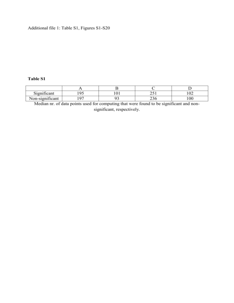
Additional file 1: Table S1, Figures S1-S20
Table S1
A
B
C
D
Significant
195
101
251
102
Non-significant
197
93
236
100
Median nr. of data points used for computing that were found to be significant and nonsignificant, respectively.
Figure S1. Sign of significant genus level bacterial interactions for I1. The plot describes
the direction (βi,j in Eq.1) of highly significant interactions. Dependent variables are along the
y axis and independent variables along the x axis, i.e. if you follow the column of given genus
upward from the x-axis until you reach a coloured cell that cell indicates the effect of the
given genus (dependent) on the genus indicated on the y-axis (independent). The colour
indicates the sign (green=positive, red=negative) of interactions that were significant at the 99%
confidence level. Cells representing non-significant relationships are black. Genus names are
coloured according to phylum provenance: Black= Actinobacteria, Red= Bacteroidetes,
Green= Firmicutes, Blue=Proteobacteria, Light Blue=Tenericutes, and
Pink=Verrucomicrobia
Figure S2. Genus level bacterial interactions for I2. The heat map describes the strength
and direction (βi,j in Eq.1) of highly significant interactions. Dependent variables are along the
y axis and independent variables along the x axis, i.e. if you follow the column of given genus
upward from the x-axis until you reach a coloured cell that cell indicates the effect of the
given genus (dependent) on the genus indicated on the y-axis (independent). The colour key
on the right-hand side indicates the sign and magnitude of interactions that were significant at
the 99% confidence level. Cells representing non-significant relationships are black. Genus
names are coloured according to phylum provenance: Black= Actinobacteria, Red=
Bacteroidetes, Green= Firmicutes, Blue=Proteobacteria, Light Blue=Tenericutes, and
Pink=Verrucomicrobia
Figure S3. Sign of significant genus level bacterial interactions for I2. The plot describes
the direction (βi,j in Eq.1) of highly significant interactions. Dependent variables are along the
y axis and independent variables along the x axis, i.e. if you follow the column of given genus
upward from the x-axis until you reach a coloured cell that cell indicates the effect of the
given genus (dependent) on the genus indicated on the y-axis (independent). The colour
indicates the sign (green=positive, red=negative) of interactions that were significant at the 99%
confidence level. Cells representing non-significant relationships are black. Genus names are
coloured according to phylum provenance: Black= Actinobacteria, Red= Bacteroidetes,
Green= Firmicutes, Blue=Proteobacteria, Light Blue=Tenericutes, and
Pink=Verrucomicrobia
Figure S4. Genus level bacterial interactions for I3. The heat map describes the strength
and direction (βi,j in Eq.1) of highly significant interactions. Dependent variables are along the
y axis and independent variables along the x axis, i.e. if you follow the column of given genus
upward from the x-axis until you reach a coloured cell that cell indicates the effect of the
given genus (dependent) on the genus indicated on the y-axis (independent). The colour key
on the right-hand side indicates the sign and magnitude of interactions that were significant at
the 99% confidence level. Cells representing non-significant relationships are black. Genus
names are coloured according to phylum provenance: Black= Actinobacteria, Red=
Bacteroidetes, Green= Firmicutes, Blue=Proteobacteria, Light Blue=Tenericutes, and
Pink=Verrucomicrobia
Figure S5. Sign of significant genus level bacterial interactions for I3. The plot describes
the direction (βi,j in Eq.1) of highly significant interactions. Dependent variables are along the
y axis and independent variables along the x axis, i.e. if you follow the column of given genus
upward from the x-axis until you reach a coloured cell that cell indicates the effect of the
given genus (dependent) on the genus indicated on the y-axis (independent). The colour
indicates the sign (green=positive, red=negative) of interactions that were significant at the 99%
confidence level. Cells representing non-significant relationships are black. Genus names are
coloured according to phylum provenance: Black= Actinobacteria, Red= Bacteroidetes,
Green= Firmicutes, Blue=Proteobacteria, Light Blue=Tenericutes, and
Pink=Verrucomicrobia
Figure S6. Genus level bacterial interactions for I4. The heat map describes the strength
and direction (βi,j in Eq.1) of highly significant interactions. Dependent variables are along the
y axis and independent variables along the x axis, i.e. if you follow the column of given genus
upward from the x-axis until you reach a coloured cell that cell indicates the effect of the
given genus (dependent) on the genus indicated on the y-axis (independent). The colour key
on the right-hand side indicates the sign and magnitude of interactions that were significant at
the 99% confidence level. Cells representing non-significant relationships are black. Genus
names are coloured according to phylum provenance: Black= Actinobacteria, Red=
Bacteroidetes, Green= Firmicutes, Blue=Proteobacteria, Light Blue=Tenericutes, and
Pink=Verrucomicrobia
Figure S7. Sign of significant genus level bacterial interactions for I4. The plot describes
the direction (βi,j in Eq.1) of highly significant interactions. Dependent variables are along the
y axis and independent variables along the x axis, i.e. if you follow the column of given genus
upward from the x-axis until you reach a coloured cell that cell indicates the effect of the
given genus (dependent) on the genus indicated on the y-axis (independent). The colour
indicates the sign (green=positive, red=negative) of interactions that were significant at the 99%
confidence level. Cells representing non-significant relationships are black. Genus names are
coloured according to phylum provenance: Black= Actinobacteria, Red= Bacteroidetes,
Green= Firmicutes, Blue=Proteobacteria, Light Blue=Tenericutes, and
Pink=Verrucomicrobia
Figure S8. Histograms of nr. data points used for computing time series regression models for
I1 (A), I2 (B), I3 (C) and I4 (D). Models based on fewer than 50 paired observations were
excluded from further analysis.
Figure S9. Effects of the number of data points used to estimate time series regression models.
The y-axes show the correlation between regression coefficients computed using the full data
sets and models using the number of data points specified on the x-axes. The full models
(Table 2) have been included in the graphs for interpretability (leftmost points). Panels A-D
represent results for I1-I4, respectively.
Figure S10. Effects of the number of data points used to estimate time series regression
models. The y-axes show the proportions of significant interactions relative to the total
number of potential interactions (square of interaction matrix dimensions), computed using
the full data sets and models using the number of data points specified on the x-axes. The full
models (Table 2) have been included in the graphs for interpretability (leftmost points). All
the relationships are highly significant (P<0.01 for all regression models). Panels A-D
represent results for I1-I4, respectively.
Figure S11. Counts of observed cases of cooperation (+/+), competition (-/-), commensalism
(+/0) and amensalism (-/0). Panels A-D represent results for I1-I4, respectively.
Figure S12. Relationship between regression coefficients computed from time series models
and contemporaneous Spearman correlations representing co-occurrence of observed taxa.
Regression lines were computed from generalized additive models using 3 degrees of freedom.
All the models except B (I2) showed significant non-linearities. All models were highly
significant (P < 0.001). Panels A-D represent results for I1-I4, respectively.
Figure S13. Genus level degree of connectedness in I2. The bar charts show the total
number of significant negative and positive genus level interactions. Dependent (acted upon)
interactions are shown in panel A while independent (acting on) interactions are in panel B.
Genus names are coloured according to phylum provenance: Black= Actinobacteria, Red=
Bacteroidetes, Green= Firmicutes, Blue=Proteobacteria, Light Blue=Tenericutes, and
Pink=Verrucomicrobia.
Figure S14. Genus level degree of connectedness in I3. The bar charts show the total
number of significant negative and positive genus level interactions. Dependent (acted upon)
interactions are shown in panel A while independent (acting on) interactions are in panel B.
Genus names are coloured according to phylum provenance: Black= Actinobacteria, Red=
Bacteroidetes, Green= Firmicutes, Blue=Proteobacteria, Light Blue=Tenericutes, and
Pink=Verrucomicrobia.
Figure S15. Genus level degree of connectedness in I4. The bar charts show the total
number of significant negative and positive genus level interactions. Dependent (acted upon)
interactions are shown in panel A while independent (acting on) interactions are in panel B.
Genus names are coloured according to phylum provenance: Black= Actinobacteria, Red=
Bacteroidetes, Green= Firmicutes, Blue=Proteobacteria, Light Blue=Tenericutes, and
Pink=Verrucomicrobia.
Figure S16. Total and mean connectedness of six main phyla estimated by time series
analysis and RE. Panels A-D show counts of positive and negative interactions significant at
the 99% confidence level estimated by time series analysis for I1-4, respectively. Panel E
shows summed competition and complementarity indices estimated by RE within the main
phyla identified in the time series studies. Panels F-I show the mean connectedness of the
phyla, i.e. the counts in A-D divided by the number of observed genera within the respective
phyla in each individual. Panel J is the numbers in E divided by the number of observed
genera within the respective phyla (see methods).
Figure S17.Within-individual relationship between relative abundance of Actinobacteria
and total community diversity (Shannon index). In each individual there was a highly
significant positive association (p<<0.001).
Figure S18. Heat map of net interaction indices estimated by RE. The plotted values are
differences between complementarity and competitive indices. More competitive interactions
were observed within than between phyla (p<<0.001). Dependent variables are along the y
axis and independent variables along the x axis, i.e. if you follow the column of given genus
upward from the x-axis until you reach a coloured cell that cell indicates the effect of the
given genus (dependent) on the genus indicated on the y-axis (independent). The colour key
on the right-hand side indicates the sign and magnitude of interactions. Species names are
coloured according to phylum provenance: Black= Actinobacteria, Red= Bacteroidetes,
Green= Firmicutes, Blue=Proteobacteria, Light Blue=Tenericutes, and
Pink=Verrucomicrobia.
Figure S19. Relative abundances in of genus level OTU’s of Bacteroides, Prevotella,
Ruminococcus and family level combinations of Lachnospiracia and Blautia. These
groups are commonly used for enterotype classification. Panels A-D show data for I1-4,
respectively. In I4 Prevotella was observed at such low abundances that the group was
removed by our filtering criteria.
Figure S20. Prevotella (A) and Bacteroides (B) relative abundances plotted as smoothed
averages along a moving window of 15 data points. High Prevotella abundances are
associated with enterotype 2. There was some evidence of temporal clustering of enterotype 2
observations (p=0.015, Wald-Wolfowitz test).